Pre-processing
Ha Tran
02/09/2021
Last updated: 2025-11-27
Checks: 7 0
Knit directory: 5_gd_Tcell/1_analysis/
This reproducible R Markdown analysis was created with workflowr (version 1.7.2). The Checks tab describes the reproducibility checks that were applied when the results were created. The Past versions tab lists the development history.
Great! Since the R Markdown file has been committed to the Git repository, you know the exact version of the code that produced these results.
Great job! The global environment was empty. Objects defined in the global environment can affect the analysis in your R Markdown file in unknown ways. For reproduciblity it’s best to always run the code in an empty environment.
The command set.seed(12345) was run prior to running the
code in the R Markdown file. Setting a seed ensures that any results
that rely on randomness, e.g. subsampling or permutations, are
reproducible.
Great job! Recording the operating system, R version, and package versions is critical for reproducibility.
Nice! There were no cached chunks for this analysis, so you can be confident that you successfully produced the results during this run.
Great job! Using relative paths to the files within your workflowr project makes it easier to run your code on other machines.
Great! You are using Git for version control. Tracking code development and connecting the code version to the results is critical for reproducibility.
The results in this page were generated with repository version b9f184a. See the Past versions tab to see a history of the changes made to the R Markdown and HTML files.
Note that you need to be careful to ensure that all relevant files for
the analysis have been committed to Git prior to generating the results
(you can use wflow_publish or
wflow_git_commit). workflowr only checks the R Markdown
file, but you know if there are other scripts or data files that it
depends on. Below is the status of the Git repository when the results
were generated:
Ignored files:
    Ignored:    .Rhistory
    Ignored:    .Rproj.user/

Untracked files:
    Untracked:  .DS_Store
    Untracked:  figure/scatter2-1.png
    Untracked:  figure/scatter3-1.png
    Untracked:  figure/scatter4-1.png
    Untracked:  figure/scatter5-1.png
    Untracked:  figure/scatter_3d4-1.png
    Untracked:  figure/scatter_interactive4-1.png
    Untracked:  figure/treemap2-1.png
    Untracked:  figure/treemap3-1.png
    Untracked:  figure/treemap4-1.png
    Untracked:  figure/treemap5-1.png

Unstaged changes:
    Modified:   0_data/RDS_plots/go_combined_dotPlot.rds
    Modified:   0_data/RDS_plots/go_combined_parTerm_dotPlot.rds
    Modified:   0_data/RDS_plots/go_dotPlot.rds
    Modified:   0_data/RDS_plots/go_parTerm_dotPlot.rds
    Modified:   0_data/RDS_plots/go_parTerm_scatter.rds
    Modified:   0_data/RDS_plots/kegg_dotPlot.rds
    Modified:   0_data/RDS_plots/kegg_path_Hmap.rds
    Modified:   0_data/RDS_plots/ma_plots.rds
    Modified:   0_data/RDS_plots/react_combined_dotPlot.rds
    Modified:   0_data/RDS_plots/react_dotPlot.rds
    Modified:   0_data/RDS_plots/vol_plots.rds
    Modified:   2_plots/1_QC/PC1_PC2.svg
    Modified:   2_plots/1_QC/PC1_PC3.svg
    Modified:   2_plots/1_QC/PC2_PC3.svg
    Modified:   2_plots/2_DE/heat_down_INT vs CONT.svg
    Modified:   2_plots/2_DE/heat_down_INT vs SVX_VAS.svg
    Modified:   2_plots/2_DE/heat_down_INT vs VAS.svg
    Modified:   2_plots/2_DE/heat_down_SVX vs SVX_VAS.svg
    Modified:   2_plots/2_DE/heat_down_SVX_VAS vs CONT.svg
    Modified:   2_plots/2_DE/heat_down_VAS vs SVX_VAS.svg
    Modified:   2_plots/2_DE/heat_up_INT vs CONT.svg
    Modified:   2_plots/2_DE/heat_up_INT vs SVX_VAS.svg
    Modified:   2_plots/2_DE/heat_up_INT vs VAS.svg
    Modified:   2_plots/2_DE/heat_up_SVX vs SVX_VAS.svg
    Modified:   2_plots/2_DE/heat_up_SVX_VAS vs CONT.svg
    Modified:   2_plots/2_DE/heat_up_VAS vs SVX_VAS.svg
    Modified:   2_plots/2_DE/hist_INT vs CONT.svg
    Modified:   2_plots/2_DE/hist_INT vs SVX_VAS.svg
    Modified:   2_plots/2_DE/hist_INT vs VAS.svg
    Modified:   2_plots/2_DE/hist_SVX vs SVX_VAS.svg
    Modified:   2_plots/2_DE/hist_SVX_VAS vs CONT.svg
    Modified:   2_plots/2_DE/hist_VAS vs SVX_VAS.svg
    Modified:   2_plots/3_FA/go/combine_go_dot.svg
    Modified:   2_plots/3_FA/go/parTerm_dot_INT vs CONT.svg
    Modified:   2_plots/3_FA/go/parTerm_dot_INT vs SVX_VAS.svg
    Modified:   2_plots/3_FA/go/parTerm_dot_SVX vs SVX_VAS.svg
    Modified:   2_plots/3_FA/go/parTerm_dot_SVX_VAS vs CONT.svg
    Modified:   2_plots/3_FA/go/parTerm_dot_VAS vs SVX_VAS.svg
    Modified:   2_plots/3_FA/go/semSim_dendrogram_INT vs CONT.svg
    Modified:   2_plots/3_FA/go/semSim_dendrogram_INT vs SVX_VAS.svg
    Modified:   2_plots/3_FA/go/semSim_dendrogram_SVX vs SVX_VAS.svg
    Modified:   2_plots/3_FA/go/semSim_dendrogram_SVX_VAS vs CONT.svg
    Modified:   2_plots/3_FA/go/semSim_dendrogram_VAS vs SVX_VAS.svg
    Modified:   2_plots/3_FA/go/semSim_scatter_INT vs CONT.svg
    Modified:   2_plots/3_FA/go/semSim_scatter_INT vs SVX_VAS.svg
    Modified:   2_plots/3_FA/go/semSim_scatter_SVX vs SVX_VAS.svg
    Modified:   2_plots/3_FA/go/semSim_scatter_SVX_VAS vs CONT.svg
    Modified:   2_plots/3_FA/kegg/combine_kegg_dot.svg
    Modified:   2_plots/3_FA/kegg/heat_Neutrophil extracellular trap formation.svg
    Modified:   2_plots/3_FA/kegg/heat_PD-L1 expression and PD-1 checkpoint pathway in cancer.svg
    Modified:   2_plots/3_FA/kegg/heat_T cell receptor signaling pathway.svg
    Modified:   2_plots/3_FA/kegg/heat_Th1 and Th2 cell differentiation.svg
    Modified:   2_plots/3_FA/kegg/heat_Th17 cell differentiation.svg
    Modified:   2_plots/3_FA/kegg/kegg_dot_INT vs CONT.svg
    Modified:   2_plots/3_FA/kegg/kegg_dot_INT vs SVX_VAS.svg
    Modified:   2_plots/3_FA/kegg/kegg_dot_SVX_VAS vs CONT.svg
    Modified:   2_plots/3_FA/kegg/kegg_dot_VAS vs SVX_VAS.svg
    Modified:   2_plots/3_FA/kegg/kegg_upset_INT vs CONT.svg
    Modified:   2_plots/3_FA/kegg/kegg_upset_INT vs SVX_VAS.svg
    Modified:   2_plots/3_FA/kegg/kegg_upset_SVX_VAS vs CONT.svg
    Modified:   2_plots/3_FA/kegg/kegg_upset_VAS vs SVX_VAS.svg
    Modified:   2_plots/3_FA/reactome/combine_react_dot.svg
    Modified:   2_plots/3_FA/reactome/react_dot_INT vs CONT.svg
    Modified:   2_plots/3_FA/reactome/react_dot_INT vs SVX_VAS.svg
    Modified:   2_plots/3_FA/reactome/react_dot_INT vs VAS.svg
    Modified:   2_plots/3_FA/reactome/react_dot_SVX vs SVX_VAS.svg
    Modified:   2_plots/3_FA/reactome/react_dot_SVX_VAS vs CONT.svg
    Modified:   2_plots/3_FA/reactome/react_dot_VAS vs SVX_VAS.svg
    Modified:   2_plots/3_FA/reactome/react_upset_INT vs CONT.svg
    Modified:   2_plots/3_FA/reactome/react_upset_INT vs SVX_VAS.svg
    Modified:   2_plots/3_FA/reactome/react_upset_INT vs VAS.svg
    Modified:   2_plots/3_FA/reactome/react_upset_SVX vs SVX_VAS.svg
    Modified:   2_plots/3_FA/reactome/react_upset_SVX_VAS vs CONT.svg
    Modified:   2_plots/3_FA/reactome/react_upset_VAS vs SVX_VAS.svg
    Modified:   2_plots/4_paper/subset_degs.svg
    Modified:   2_plots/combine_ipa_dot.svg
    Modified:   2_plots/dnf_plot.svg
    Modified:   2_plots/intVsvxVAS.svg
    Modified:   2_plots/upstream_hmap.svg
    Modified:   3_output/DEGs.xlsx
    Modified:   3_output/Gene Ontology.xlsx
    Modified:   3_output/KEGG.xlsx
    Modified:   3_output/Reactome.xlsx
    Modified:   3_output/deg_all_new.xlsx
    Modified:   3_output/deg_sig_new.xlsx
    Modified:   3_output/eigenvalues.xlsx
    Modified:   3_output/enrichKEGG_sig.xlsx
    Modified:   3_output/reactome_all_new.xlsx
    Modified:   3_output/reactome_sig_new.xlsx
    Modified:   3_output/semSim_GO_sig.xlsx
    Modified:   README.html
    Modified:   README.md
    Modified:   figure/dot2-1.png
    Modified:   figure/dot3-1.png
    Modified:   figure/dot4-1.png
    Modified:   figure/dot5-1.png
    Modified:   figure/upset2-1.png
    Modified:   figure/upset3-1.png
    Modified:   figure/upset4-1.png
    Modified:   figure/upset5-1.png
Note that any generated files, e.g. HTML, png, CSS, etc., are not included in this status report because it is ok for generated content to have uncommitted changes.
These are the previous versions of the repository in which changes were
made to the R Markdown (1_analysis/setUp.Rmd) and HTML
(docs/setUp.html) files. If you’ve configured a remote Git
repository (see ?wflow_git_remote), click on the hyperlinks
in the table below to view the files as they were in that past version.
| File | Version | Author | Date | Message |
|---|---|---|---|---|
| html | d519e7f | Ha Tran | 2024-12-03 | Build site. |
| html | 5dce909 | Ha Tran | 2024-11-07 | Build site. |
| html | d71eeb4 | Ha Tran | 2024-10-16 | Build site. |
| Rmd | 5f0c7a1 | Ha Tran | 2024-10-16 | workflowr::wflow_publish(here::here("1_analysis/*.Rmd")) |
| html | ae93fcc | tranmanhha135 | 2024-02-02 | Build site. |
| Rmd | fbcdd69 | tranmanhha135 | 2024-02-02 | workflowr::wflow_publish(here::here("1_analysis/*.Rmd")) |
| Rmd | ccb39d7 | tranmanhha135 | 2022-10-22 | safety commit |
| html | 2c24612 | tranmanhha135 | 2022-10-13 | build website |
| Rmd | 866017e | tranmanhha135 | 2022-10-13 | minor changes |
| Rmd | 324032b | tranmanhha135 | 2022-10-11 | resize images |
| Rmd | 43675d3 | tranmanhha135 | 2022-10-06 | Add IPA data |
| html | 43675d3 | tranmanhha135 | 2022-10-06 | Add IPA data |
| html | 11a5cf4 | tranmanhha135 | 2022-10-03 | build wedsite |
| Rmd | 1101367 | tranmanhha135 | 2022-10-02 | Completed functional enrichment for all comparison |
| html | 1101367 | tranmanhha135 | 2022-10-02 | Completed functional enrichment for all comparison |
| html | 68585df | tranmanhha135 | 2022-09-20 | build webste |
| html | 6b987dc | tranmanhha135 | 2022-09-08 | Build site. |
| html | b9caf15 | tranmanhha135 | 2022-09-08 | Build site. |
| html | 0df047f | tranmanhha135 | 2022-09-08 | minor changes to build and publish |
| Rmd | 959a5df | tranmanhha135 | 2022-09-07 | rewrite after conversation with Jimmy |
| html | 959a5df | tranmanhha135 | 2022-09-07 | rewrite after conversation with Jimmy |
| html | 54e0166 | Ha Manh Tran | 2022-01-01 | Build site. |
| html | 32454d5 | Ha Manh Tran | 2022-01-01 | Build site. |
| Rmd | c667dd0 | Ha Manh Tran | 2022-01-01 | workflowr::wflow_publish(files = here::here(c("1_analysis/index.Rmd", |
| Rmd | 3b268fc | Ha Tran | 2021-12-09 | multiple FC, reactome, big clean up. |
| html | 3b268fc | Ha Tran | 2021-12-09 | multiple FC, reactome, big clean up. |
| html | 7247e9c | Ha Tran | 2021-11-30 | additional KEGG heatmap, pathview, reactome |
| html | f4ba25b | Ha Manh Tran | 2021-11-23 | Build site. |
| html | 516f8e9 | Ha Tran | 2021-11-18 | changed treat lfc to from 0.584 to 1 |
| Rmd | 8092dd7 | Ha Tran | 2021-11-04 | initial commit |
| html | 8092dd7 | Ha Tran | 2021-11-04 | initial commit |
Data Setup
Prior to this analysis, reads were:
Trimmed using
AdapterRemovalAligned to GRCm38/mm10 using
STARReads quantification peforemd with
featureCounts
Transcript QC, alignment, and quantification were performed by Dr Jimmy Breen
# working with data
# working with data
library(dplyr)
library(magrittr)
library(readr)
library(tibble)
library(reshape2)
library(tidyverse)
library(bookdown)
library(here)
library(scales)

# Visualisation:
library(ggbiplot)
library(ggrepel)
library(grid)
library(corrplot)
library(DT)
library(plotly)
library(patchwork)

# Bioconductor packages:
library(AnnotationHub)
library(edgeR)
library(limma)
library(Glimma)

# Fontlib
library(extrafont)
rawCount <- readRDS(here::here("0_data/RDS_objects/rawCount.rds"))
DT <- readRDS(here::here("0_data/functions/DT.rds"))
# to increase the knitting speed. change to T to save all plots
savePlots <- F
# Theme
bossTheme <- readRDS(here::here("0_data/functions/bossTheme.rds"))
bossTheme_bar <- readRDS(here::here("0_data/functions/bossTheme_bar.rds"))
groupColour <- readRDS(here::here("0_data/functions/groupColour.rds"))
groupColour_dark <- readRDS(here::here("0_data/functions/groupColour_dark.rds"))
# Plotting
convert_to_superscript <- readRDS(here::here("0_data/functions/convert_to_superscript.rds"))
exponent <- readRDS(here::here("0_data/functions/exponent.rds"))
format_y_axis <- readRDS(here::here("0_data/functions/format_y_axis.rds"))Import Raw Count Data
To save time, this will only be performed once at the begining of the analysis. For subsequent analysis, the file will just be loaded.
Due to the unusual library size, control 3 was removed from the analysis
# import the mergedOnly dataset, provided by Dr Jimmy Breen on the 24/09/21
rawCount <- read_tsv(here::here("0_data/raw_data/allSamples_mergedOnly.featureCounts.txt"),
                     col_names = TRUE,
                     comment = "#") %>%
  dplyr::rename(CONT1 = "../2_Hisat2_merged/CONT1_ATGTCA_merged.sorted.nodup.bam",
                CONT2 = "../2_Hisat2_merged/CONT2_CGATGT_merged.sorted.nodup.bam",
                CONT4 = "../2_Hisat2_merged/CONT4_ACTTGA_merged.sorted.nodup.bam",
                INT1 = "../2_Hisat2_merged/INT1_GTCCGC_merged.sorted.nodup.bam",
                INT2 = "../2_Hisat2_merged/INT2_ACAGTG_merged.sorted.nodup.bam",
                INT3 = "../2_Hisat2_merged/INT3_GATCAG_merged.sorted.nodup.bam",
                INT4 = "../2_Hisat2_merged/INT4_CTTGTA_merged.sorted.nodup.bam",
                SVX1 = "../2_Hisat2_merged/SVX1_GTTTCG_merged.sorted.nodup.bam",
                SVX2 = "../2_Hisat2_merged/SVX2_TAGCTT_merged.sorted.nodup.bam",
                SVX3 = "../2_Hisat2_merged/SVX3_ATCACG_merged.sorted.nodup.bam",
                SVX4 = "../2_Hisat2_merged/SVX4_GCCAAT_merged.sorted.nodup.bam",
                SVX_VAS1 = "../2_Hisat2_merged/SVX_VAS1_AGTCAA_merged.sorted.nodup.bam",
                SVX_VAS2 = "../2_Hisat2_merged/SVX_VAS2_AGTTCC_merged.sorted.nodup.bam",
                SVX_VAS3 = "../2_Hisat2_merged/SVX_VAS3_TGACCA_merged.sorted.nodup.bam",
                SVX_VAS4 = "../2_Hisat2_merged/SVX_VAS4_GGCTAC_merged.sorted.nodup.bam",
                VAS1 = "../2_Hisat2_merged/VAS1_CAGATC_merged.sorted.nodup.bam",
                VAS2 = "../2_Hisat2_merged/VAS2_GTGAAA_merged.sorted.nodup.bam",
                VAS3 = "../2_Hisat2_merged/VAS3_GTGGCC_merged.sorted.nodup.bam",
                VAS4 = "../2_Hisat2_merged/VAS4_CCGTCC_merged.sorted.nodup.bam",) %>%
  column_to_rownames("Geneid") %>%
  as.data.frame()
  rownames(rawCount) <- gsub("\\..+$", "", rownames(rawCount))

# Removing the non-numerical metadata column. SVX_VAS1 may also be an outlier, it is number 18 (BTW)
rawCount<- rawCount[, c(6,7,9:25)]

saveRDS(rawCount, here::here("0_data/RDS_objects/rawCount.rds"))
Import Metadata
There are generally two metadata required for DGE analysis.
metadata about each sample
metadata about each gene
Sample Metadata
The sample metadata can be extracted from the logCPM
column names. These data include sample_id,
sample_group, sample_type.
The sample metadata will be manually generated and stored in the
/0_data/raw_data/ directory.
samples <- read_tsv(here::here("0_data/raw_data/samples.tsv"),
                    col_names = TRUE) %>%
  column_to_rownames("1")
Gene Metadata
Gene annotation is useful for the DGE analysis as it will provide useful information about the genes. The annotated genes of Mus musculus can be pulled down by using Annotation Hub.
Annotation Hub also has a web service that can be assessed through
the display function. Pulling down the gene annotation can take a long
time, so after the initial run, the annotated genes is saved to a
genes.rds file. To save time, if genes.rds is
already present, don’t run the code chunk.
ah <- AnnotationHub()
ah %>%
  subset(grepl("musculus", species)) %>%
  subset(rdataclass == "EnsDb")

#viewing web service for annotation hub
#d <- display(ah)

# Annotation hub html site was used to identify 'code' for the lastest mouse genome from Ensembl
ensDb <- ah[["AH95775"]]

genes <- genes(ensDb) %>%
  as.data.frame()

#the annotated genes are saved into a RDS object to save computational time in subsequent run of the setUp.Rmd
genes %>% saveRDS(here::here("0_data/RDS_objects/gene_metadata.rds"))
Using the annotated gene list through AnnotationHub(), load into
object called geneMeta. Filter out all genes that are
present in the rawCount and display the number of unique gene_biotypes
present in the rawCount and geneMeta
geneMeta <- read_rds(here::here("0_data/RDS_objects/gene_metadata.rds"))

#prepare the gene data frame to contain the genes listed in the rownames of 'rawCount' data
geneMeta <- data.frame(gene = rownames(rawCount)) %>%
  left_join(geneMeta %>% as.data.frame,
            by = c("gene"="gene_id")) %>%
  dplyr::distinct(gene, .keep_all=TRUE)

rownames(geneMeta) <- geneMeta$gene

#Using the table function, the details of the genes present in the rawCount data can be summaried.
genes <- geneMeta$gene_biotype %>% table %>% as.data.frame()
colnames(genes) <- c("Gene Biotype", "Frequency")
genes$`Gene Biotype` <- as.character(genes$`Gene Biotype`)
genes$`Gene Biotype`[grep("_", genes$`Gene Biotype`)] <- str_to_sentence(str_replace_all(genes$`Gene Biotype`[grep("_", genes$`Gene Biotype`)], "_", " "))
Interactive pie chart
pie <- plot_ly(genes, labels = ~`Gene Biotype`, values = ~`Frequency`, type = 'pie',
               textposition = 'inside',
               textinfo = 'label+percent',
               # insidetextfont = list(color = '#FFFFFF'),
               hoverinfo = 'text',
               text = ~paste(`Frequency`, ' genes'),
               marker = list(colors = colors,line = list(color = '#FFFFFF', width = 1)),
               #The 'pull' attribute can also be used to create space between the sectors
        showlegend = T)
pie <- pie %>% layout(title = 'Frequency of gene biotype',
         xaxis = list(showgrid = FALSE, zeroline = FALSE, showticklabels = FALSE),
         yaxis = list(showgrid = FALSE, zeroline = FALSE, showticklabels = FALSE))

pie
Table
genes %>% DT(.,caption = "Table 1: Gene biotype")Create DGEList object
Digital Gene Expression List (DGElist) is a R object class often used for differential gene expression analysis as it simplifies plotting, and interaction with data and metadata.
The DGEList object holds the three dataset that have
imported/created, including rawCount data and
sampleMetadata and geneMeta metadata.
To further save time and memory, genes that were not expressed
acrossed all samples (i.e., 0 count across all columns) are
all removed
#Create DGElist with rawCOunt and gene data. Remove all genes with 0 expression in all treatment groups
dge <- DGEList(counts = rawCount,
               samples = samples,
               genes = geneMeta,
               remove.zeros = TRUE
               )

dge$samples$group <- factor(dge$samples$group, levels = c("CONT", "INT", "SVX", "VAS", "SVX_VAS"))
Pre-processing and QC
Pre-processing steps increased the power of the downstream DGE analysis by eliminating majority of unwanted variance that could obscure the true variance caused by the differences in sample conditions. There are several standard steps that are commonly followed to pre-process and QC raw read counts, including:
Checking Library Size
Removal of Undetectable Genes
Normalisation
QC through MDS/PCA
Checking Library Size
A simple pre-processing/QC step is checking the quality of library
size (total number of mapped and quantified reads) for each treatment.
This enable identification of potentially mis-labeled or outlying
samples. This is often visualised through ggplot.
custom_labels <- function(data, y, x) {
  exp <- exponent(df = data,y_column = y)
  ifelse(x >= 1000 | x<= 0.001 & x!=0, {
    l <- x / 10^exp
    parse(text=l)
  }, format(x, scientific = FALSE))
}

libSize <- ggplot(dge$samples,aes(x = sample, y = lib.size, fill = group)) +
  geom_col(width = 0.8) +
  geom_hline(aes(yintercept = lib.size), data = . %>% summarise_at(vars(lib.size), mean), linetype = 2) +
  scale_y_continuous(expand = expansion(mult = c(0, 0)),
                     labels = function(x) custom_labels(data = dge$samples, y = "lib.size", x = x)) +
  scale_fill_manual(values = groupColour)+
  labs(x = "",
       title = "Sample Library Size",
       y = paste0("Library size (\u00D710", convert_to_superscript(exponent(dge$samples, "lib.size")), ")")) +
  coord_flip() +
  bossTheme_bar(base_size = 14)

libSize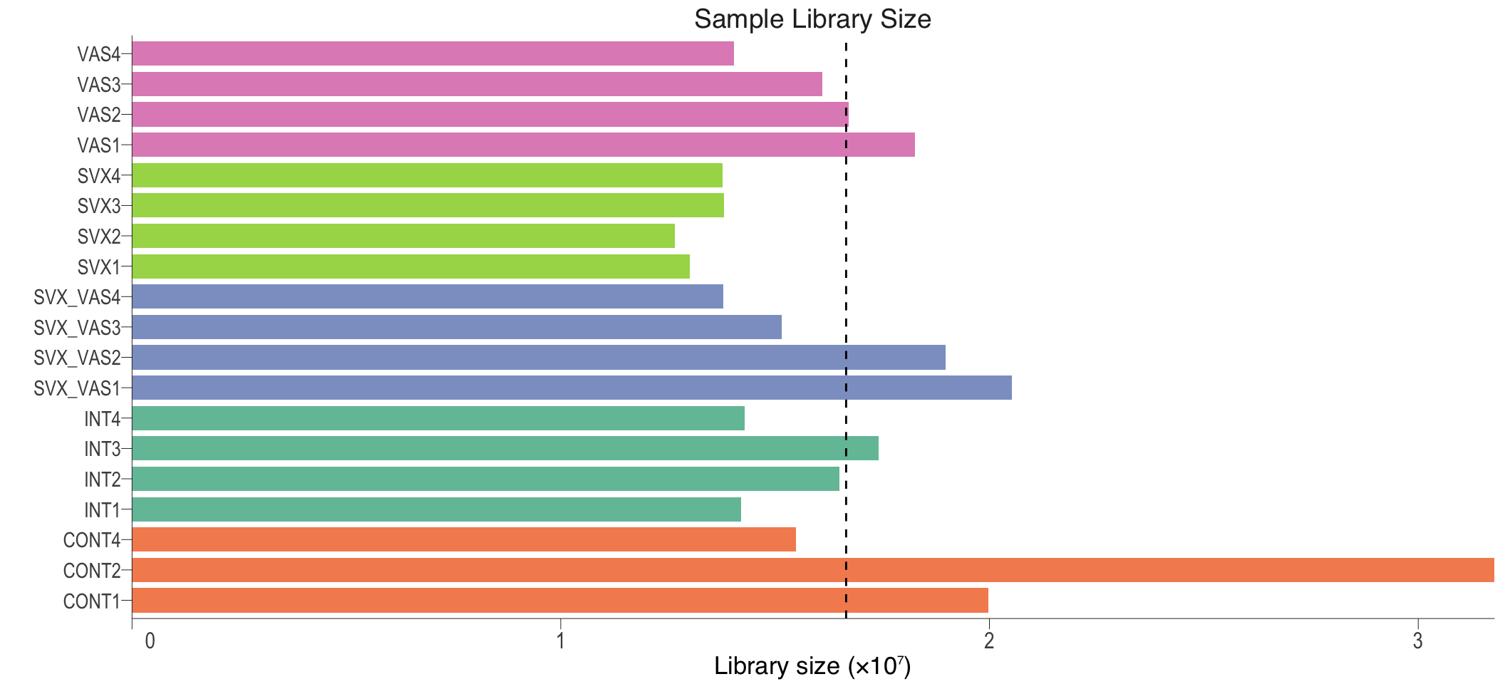
Sample library size. Dash line represent average library size
if(savePlots){
  ggsave(here::here("2_plots/1_QC/library_size.svg"),
         plot = libSize,
         width = 10,
         height = 9,
         units = "cm")
}
Removal of Low-Expressed Genes
Filtering out low-expressed genes is a standard pre-processing step in DGE analysis as it can significantly increase the power to differentiate differentially expressed genes by eliminating the variance caused by genes that are lowly expressed in all samples.
The threshold of removal is arbitrary and is often determined after
visualisation of the count distribution. The count distribution can be
illustrated in a density plot through ggplot. A common
metric used to display the count distribution is log Counts per
Million (logCPM)
cpm_filter <- 1.5
beforeFiltering <- dge %>%
  edgeR::cpm(log = TRUE) %>%
  melt %>%
  dplyr::filter(is.finite(value)) %>%
  ggplot(aes(x = value,colour = Var2)) +
  geom_density() +
  labs(title = "Before filtering low-expressed genes",
       subtitle = paste0(nrow(dge), " genes"),
       x = "logCPM",
       y = "Density",
       colour = "Sample Groups") +
  bossTheme_bar(base_size = 14)

if(savePlots){
  ggsave("counts_before_filtering.svg",
         plot = beforeFiltering + bossTheme(base_size = 14),
         width = 10,
         height = 10,
         units = "cm",
         path = here::here("2_plots/1_QC/"))
}
Ideally, the filtering the low-expressed genes should remove the
large peak with logCPM < 0, i.e., remove any genes which
have less than one count per million.
A common guideline is to keep all genes that have > 1-2 cpm in the
smallest group on a treatment. In this case, the smallest group is 3 as
each treatment condition had three replicates. However, due to the high
variance of some groups, the filtering is increased to keep genes that
are are more than 3 CPM in atleast 3 samples.
Mathematically this would be identifying genes (rows) with CPM
> 3; and identifying total row sum that is
>= 3.
#the genes kept have >2 CPM for at least 4 samples
keptGenes <- (rowSums(cpm(dge) > 3) >= 3)
afterFiltering <- dge %>%
  edgeR::cpm(log = TRUE) %>%
  #for var1 (gene names) extract only the keptGenes and discard all other genes in the logCPM data
  magrittr::extract(keptGenes, ) %>%
  melt %>%
  dplyr::filter(is.finite(value)) %>%
  ggplot(aes(x = value,colour = Var2)) +
  geom_density() +
  labs(title = "After filtering low-expressed genes",
       subtitle = paste0(table(keptGenes)[[2]], " genes"),
       x = "logCPM",
       y = "Density",
       colour = "Sample Groups") +
  bossTheme(base_size = 14,legend = "bottom")

if(savePlots){
  ggsave("counts_after_filtering.svg",
         plot = afterFiltering + bossTheme(base_size = 14),
         width = 10,
         height = 10,
         units = "cm",
         path = here::here("2_plots/1_QC/"))
}

beforeFiltering + afterFiltering + plot_layout(guides = "collect") & bossTheme(base_size = 14,legend = "none")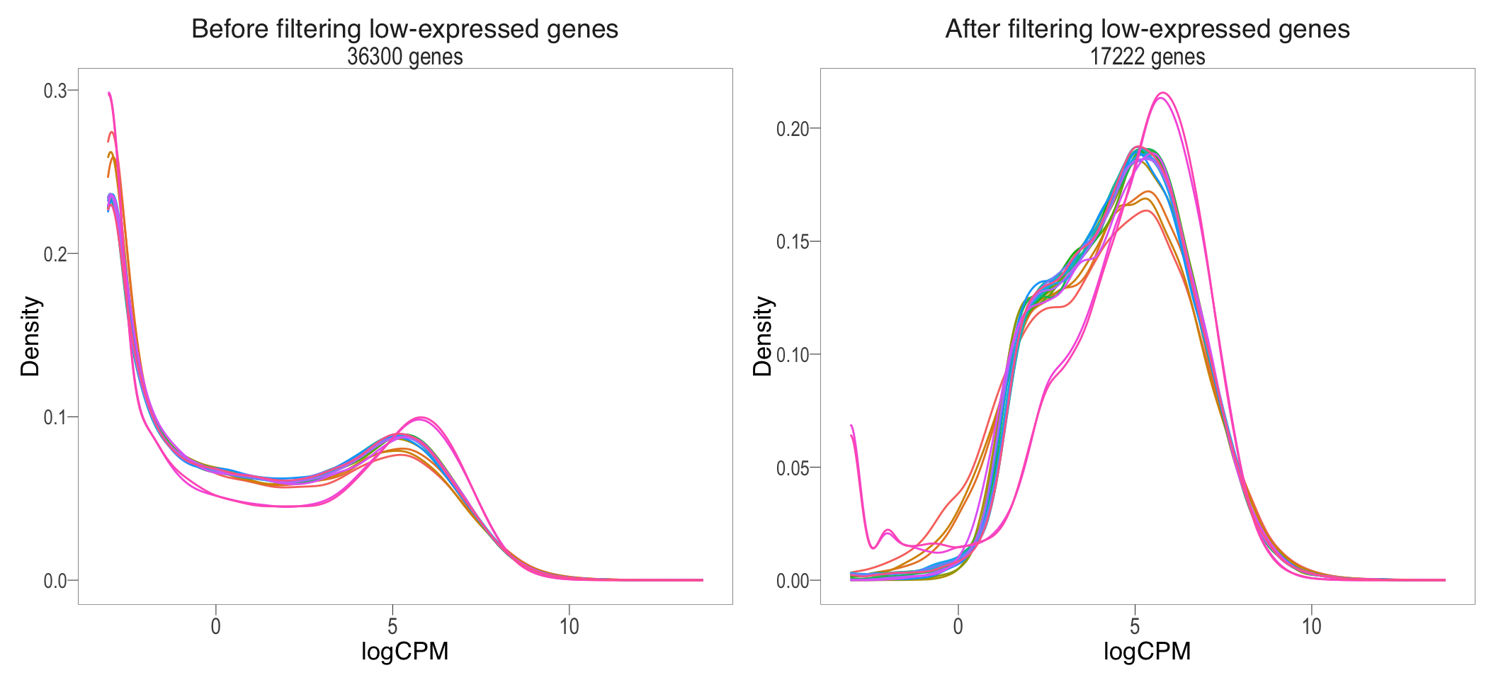
Before and after removal of lowly expressed genes
if(savePlots){
  ggsave(filename = "counts_before_after_filtering.svg",
         path = here::here("2_plots/1_QC/"),
         width = 20,
         height = 14,
         units = "cm")
}
Following the filtering of low-expressed genes < 3 CPM in at least 3 samples, out of the total 36300 genes left after the removal of genes with no expression, 19078 genes were removed, leaving only 17222 genes remaining for the downstream analysis.
Subset the DGElist object
After filtering the low-expressed genes, the DGElist object is updated to eliminate the low-expressed genes from future analysis
#extract genes from keptGenes and recalculate the lib size
dge <- dge[keptGenes,,keep.lib.sizes = FALSE]
Normalisation
Using the TMM (trimmed mean of M value) method of normalisation
through the edgeR package. The TMM approach creates a
scaling factor as an offset to be supplied to Negative Binomial model.
The ca;cNormFactors function calculate the normalisation
and return the adjusted norm.factor to the
dge$samples element.
Mean-difference (MD) plots
The following visualisation of the TMM normalisation is plotted using
the mean-difference (MD) plot. The MD plot visualise the library
size-adjusted logFC between two samples (the difference) against the
log-expression across all samples (the mean). In this instance,
sample 1 is used to compare against an artificial library
construct from the average of all the other samples
Ideally, the bulk of gene expression following the TMM normalisation
should be centred around expression log-ratio of 0, which
indicates that library size bias between samples have been successfully
removed. This should be repeated with all the samples in the dge
object.
Before
par(mfrow = c(5, 4), mar = c(2, 2, 1, 1))

for (i in 1:nrow(dge$samples)) {
  limma::plotMD(cpm(dge, log = TRUE), column = i)
  abline(h = 0, col = "red", lty = 2, lwd = 2)
}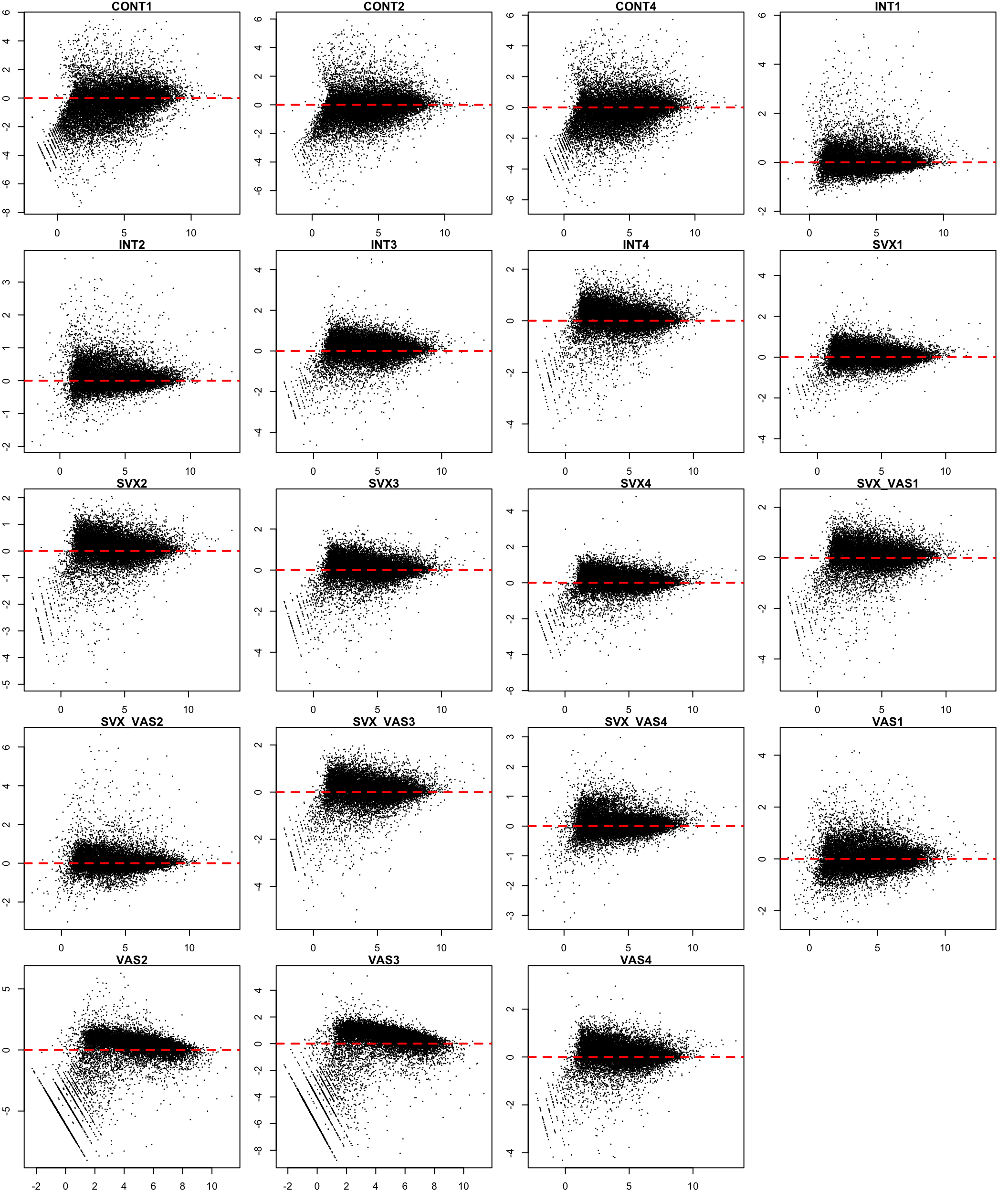
MA plot before TMM normalisation
| Version | Author | Date |
|---|---|---|
| d71eeb4 | Ha Tran | 2024-10-16 |
After
#after normalisation
dge <- edgeR::calcNormFactors(object = dge,
                              method = "TMM")

par(mfrow = c(5, 4), mar = c(2, 2, 1, 1))

for (i in 1:nrow(dge$samples)) {
  limma::plotMD(cpm(dge, log = TRUE), column = i)
  abline(h = 0, col = "red", lty = 2, lwd = 2)
}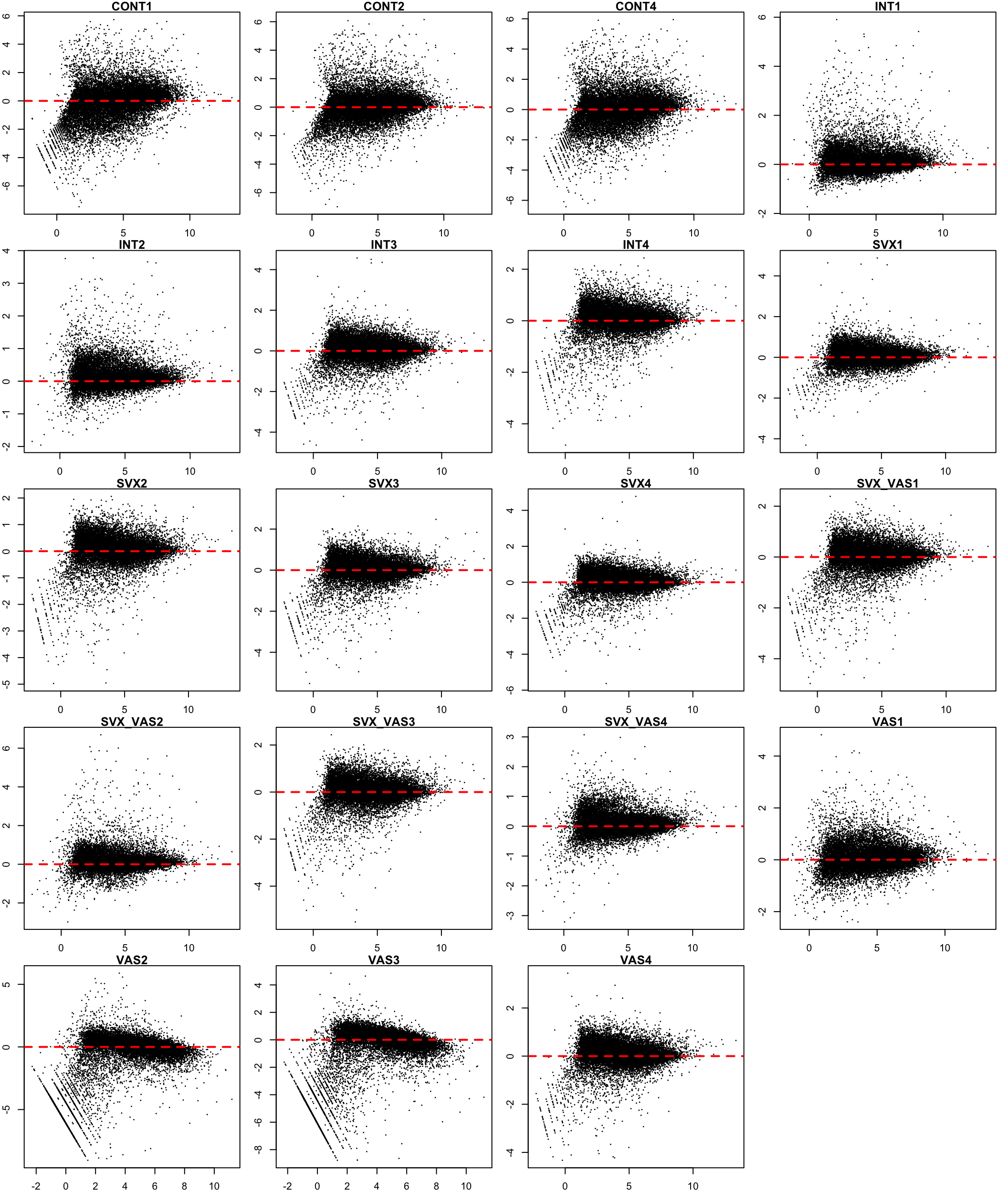
MA plot after TMM normalisation
| Version | Author | Date |
|---|---|---|
| d71eeb4 | Ha Tran | 2024-10-16 |
Normalisation factors
dge$samples %>% DT(.,caption = "Table: Normalised samples")Pinciple Component Analysis (PCA)
Principal Component Analysis (PCA) is a dimensionality reduction technique widely employed to capture the intrinsic patterns and variability within high-dimensional datasets. By transforming the original gene expression data into a set of uncorrelated principal components, PCA helps reveal the major sources of variation in the dataset. This enables assessment of overall similarity between samples
# Perform PCA analysis:
pca_analysis <- prcomp(t(cpm(dge, log = TRUE)))

# Create the plot
pca_2d <- lapply(list(`1_2` = c("PC1", "PC2"),
                      `1_3` = c("PC1", "PC3"),
                      `2_3` = c("PC2", "PC3")),
            function(i) {
              p <- pca_analysis$x %>%
                cbind(dge$samples) %>%
                as_tibble() %>%
                ggplot(aes(x = .data[[i[1]]], y = .data[[i[2]]], colour = group, shape = as.factor(rep))) +
                geom_point(size=3) +
                scale_color_manual(values = groupColour)+
                # scale_shape_manual(values = c(15:21)) +
                labs(x = paste0(i[1], " (", percent(summary(pca_analysis)$importance["Proportion of Variance",i[1]]),")"),
                     y = paste0(i[2], " (", percent(summary(pca_analysis)$importance["Proportion of Variance",i[2]]),")"),
                     colour = "Groups",
                     shape = "Replicate") +
                bossTheme(base_size = 14,legend = "right")

              ggsave(paste0(i[1], "_", i[2],".svg"), plot = p,path = here::here("2_plots/1_QC/"),width = 11, height = 9, units = "cm")
              return(p)
            })

wrap_plots(pca_2d) + plot_layout(guides = "collect") & bossTheme(base_size = 14,legend = "bottom")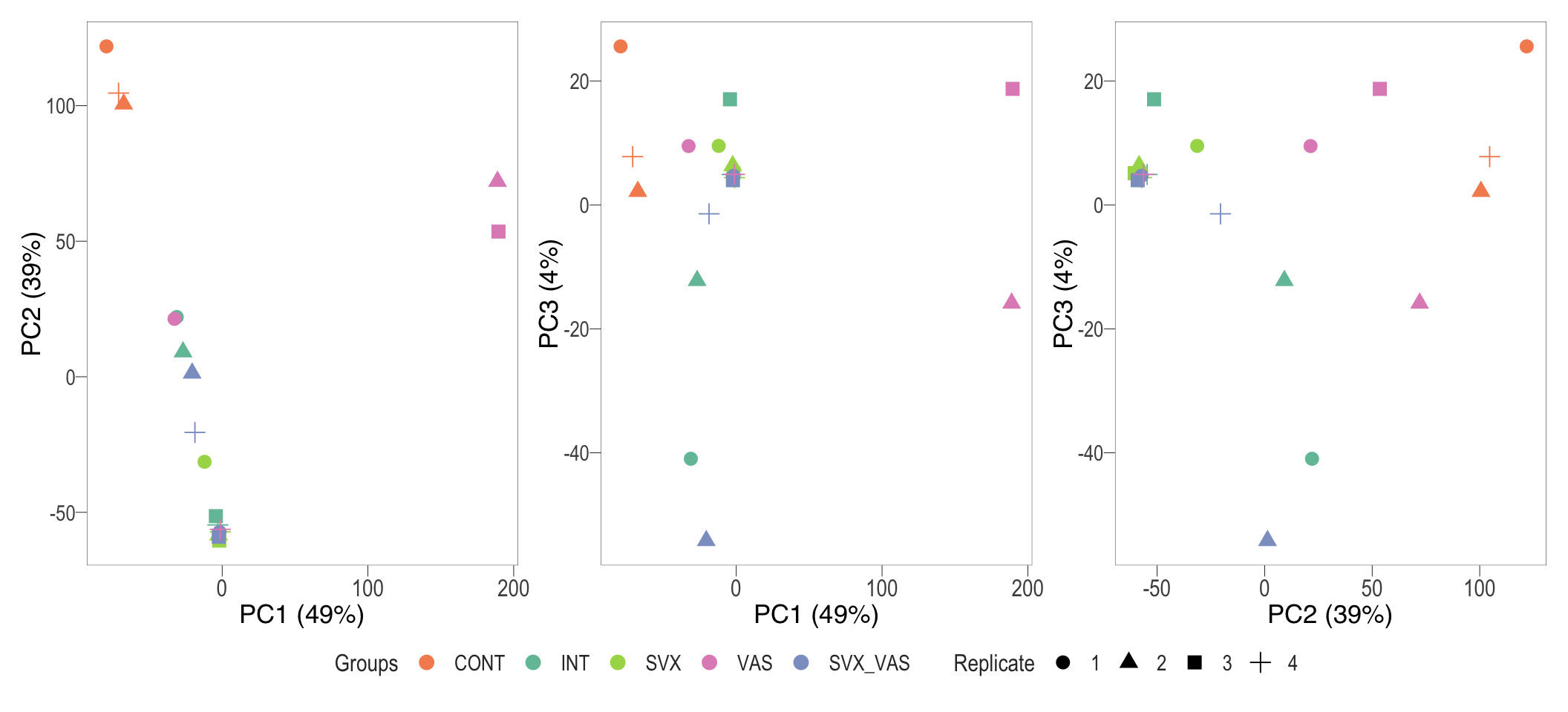
PCA plot
| Version | Author | Date |
|---|---|---|
| d71eeb4 | Ha Tran | 2024-10-16 |
| ae93fcc | tranmanhha135 | 2024-02-02 |
| 2c24612 | tranmanhha135 | 2022-10-13 |
| 1101367 | tranmanhha135 | 2022-10-02 |
| b9caf15 | tranmanhha135 | 2022-09-08 |
| 0df047f | tranmanhha135 | 2022-09-08 |
| 959a5df | tranmanhha135 | 2022-09-07 |
| 32454d5 | Ha Manh Tran | 2022-01-01 |
| 3b268fc | Ha Tran | 2021-12-09 |
| 8092dd7 | Ha Tran | 2021-11-04 |
pc <- pca_analysis[["x"]][,1:3] %>% as.data.frame()

pc$PC2 <- -pc$PC2
pc$PC3 <- -pc$PC3

pc = cbind(pc, dge$samples)

totVar <- summary(pca_analysis)[["importance"]]['Proportion of Variance',]
totVar <- 100 * sum(totVar[1:3])

pca_3d <- plot_ly(pc, x = ~PC1, y = ~PC2, z = ~PC3, color = ~dge$samples$group, colors = groupColour,
                  marker = list(symbol = 'circle', sizemode = 'diameter', size =5),
                  # sizes = c(5, 70),
                  # text = ~paste('Term    :', term,'<br>P. Term:', parentTerm, '<br>Sig       :', score),
                  hoverinfo = 'text') %>%
  layout(showlegend = T,
         title = paste0('Total Explained Variance = ', totVar),
         scene = list(xaxis = list(title = 'PC 1 (49%)',
                                   gridcolor = 'rgb(194, 197, 204)',
                                   zerolinewidth = 1,
                                   ticklen = 5,
                                   gridwidth = 2),
                      yaxis = list(title = 'PC 2 (39%)',
                                   gridcolor = 'rgb(194, 197, 204)',
                                   zerolinewidth = 1,
                                   ticklen = 5,
                                   gridwith = 2),
                      zaxis = list(title = 'PC 3 (4%)',
                                   gridcolor = 'rgb(194, 197, 204)',
                                   zerolinewidth = 1,
                                   ticklen = 5,
                                   gridwith = 2)))

pca_3d
test <- read_csv(file = here::here("c:\\Users/tranm/Documents/test.csv"))
test_pca <- prcomp(t(test))
test_plot <- test_pca$x %>%
as.data.frame() %>%
as_tibble() %>%
ggplot(aes(x = PC1, y = PC2, colour = rownames(test_pca$x))) +
geom_point(size=3, alpha=0.5) +
scale_shape_manual(values = c(15:18)) +
labs(
title = "PC1 & PC2",
x = paste0("PC1 (", percent(summary(test_pca)$importance["Proportion of Variance","PC1"]),")"),
y = paste0("PC2 (", percent(summary(test_pca)$importance["Proportion of Variance","PC2"]),")"),
colour = "Groups",
shape = "Replicates"
)
library(plotly)
ggplotly(test_plot)
ggbiplot(test_pca,choices = 1:2,
groups = rownames(test_pca$x),
ellipse = FALSE,
var.axes = FALSE,
# ellipse.prob = 0.96,
alpha = 0)+
labs(
# title = "Principle Component Analysis",
color = "Sample Group"
) +
geom_point(aes(colour = rownames(test_pca$x)), size = 2)+
theme(legend.position = "bottom",
legend.box.margin = margin(-15,0,-5,0)
# legend.key.size = unit(0, "lines")
)Unknown variation
To further investigate why the Vasectomised group is so varied, the top 1000 most variable genes from PC1 were extracted from the PCA analysis. This extraction was performed with all groups (TL) and again with only the Vasectomised group (BR). Due to the high presence of unknown genes, all non-annotated genes were removed.
######################################
### JIMMY's CODE SNIPPET

## All groups
# Extract DF of most variable PC1 genes
#
pca_VASonly <- prcomp(t(cpm(dge[,16:19], log = TRUE)), scale = FALSE)

eigen <- data.frame(sort(abs(pca_analysis$rotation[,"PC1"]), decreasing=TRUE)[1:1000])
eigen <- rownames_to_column(eigen)
colnames(eigen) <- c("gene", "PC1")
eigen <- merge(x = eigen, y = dge$genes, by="gene") %>%  dplyr::select(c("gene", "gene_name", "PC1", "gene_biotype", "description", "entrezid"))
# Remove unknown, predicted and NA genes
eigen <- eigen[!grepl("^Gm", eigen$gene_name),]
eigen <- eigen[!grepl("^RIKEN", eigen$description),]
eigen <- na.omit(eigen)
eigen <- remove_rownames(eigen) %>% column_to_rownames(var = "gene")

## only VAS group
eigen_VAS_all <- data.frame(sort(abs(pca_VASonly$rotation[,"PC1"]), decreasing=TRUE)[1:1000])
eigen_VAS_all <- rownames_to_column(eigen_VAS_all)
colnames(eigen_VAS_all) <- c("gene", "PC1")
eigen_VAS_all <- merge(x = eigen_VAS_all, y = dge$genes, by="gene") %>%  dplyr::select(c("gene", "gene_name", "PC1", "gene_biotype", "description", "entrezid"))
# Removed unknown, predicted, and NA genes
eigen_VAS <- eigen_VAS_all[!grepl("^Gm",eigen_VAS_all$gene_name),]
eigen_VAS <- eigen_VAS[!grepl("^RIKEN", eigen_VAS$description),]
eigen_VAS <- na.omit(eigen_VAS)
eigen_VAS <- remove_rownames(eigen_VAS) %>% column_to_rownames(var = "gene")

intersect <- intersect(x = eigen$gene_name, y = eigen_VAS$gene_name) %>% as.data.frame()
eigenvalues <- list(eigen_VAS_all,eigen_VAS)
names(eigenvalues) <- c("eigenvalues_PC1_VAS_all", "eigenvalues_PC1_VAS")
######################################
All groups
eigen[order(-eigen$PC1),] %>% DT(.,caption = "Most variable genes in PC1 of all groups") Vasectomised group
eigen_VAS[order(-eigen_VAS$PC1),] %>% DT(., caption = "Most variable genes in PC1 of only VAS group")Correlation plot
corr_plot <- pca_analysis$x %>%
  as.data.frame() %>%
  rownames_to_column("sample") %>%
  left_join(dge$samples) %>%
  as_tibble() %>%
  dplyr::select(
    PC1,
    PC2,
    PC3,
    Groups=group,
    Mated,
    "Library size"=lib.size,
    "Normalisation Factor"=norm.factors
  ) %>%
  mutate(Groups = as.numeric(as.factor(Groups))) %>%
  cor(method = "spearman") %>%
  corrplot(type = "lower",
           diag = FALSE,
           addCoef.col = 1, addCoefasPercent = TRUE
  )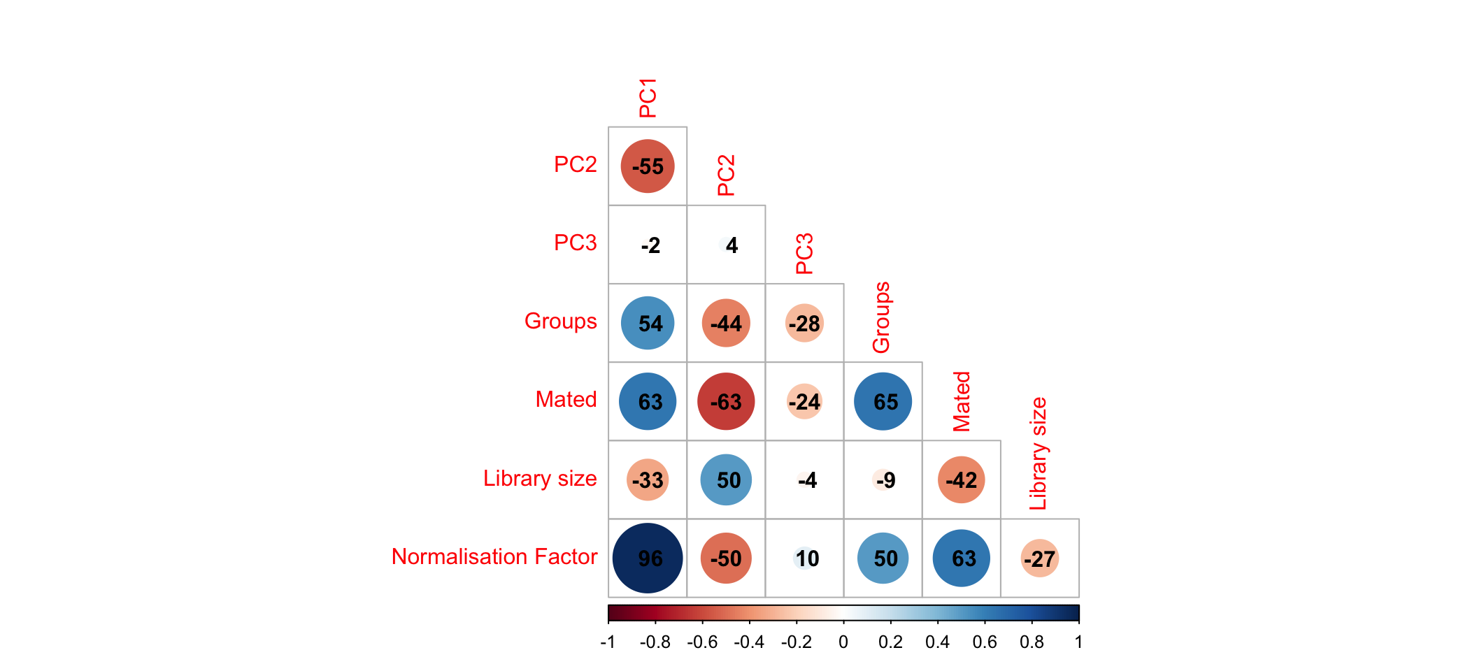
Correlation between first three principle components and measured variables
# Save DGElist object into the data/R directory
saveRDS(object = dge, file = here::here("0_data/RDS_objects/dge.rds"))

writexl::write_xlsx(eigenvalues, here::here("3_output/eigenvalues.xlsx"))
# saveRDS(object = gg_publish, file = here::here("0_data/RDS_objects/gg_publish.rds"))
sessionInfo()R version 4.4.1 (2024-06-14)
Platform: aarch64-apple-darwin20
Running under: macOS 26.1
Matrix products: default
BLAS: /Library/Frameworks/R.framework/Versions/4.4-arm64/Resources/lib/libRblas.0.dylib
LAPACK: /Library/Frameworks/R.framework/Versions/4.4-arm64/Resources/lib/libRlapack.dylib; LAPACK version 3.12.0
locale:
[1] en_US.UTF-8/en_US.UTF-8/en_US.UTF-8/C/en_US.UTF-8/en_US.UTF-8
time zone: Australia/Adelaide
tzcode source: internal
attached base packages:
[1] grid stats graphics grDevices utils datasets methods
[8] base
other attached packages:
[1] extrafont_0.19 Glimma_2.16.0 edgeR_4.4.2
[4] limma_3.62.2 AnnotationHub_3.14.0 BiocFileCache_2.14.0
[7] dbplyr_2.5.1 BiocGenerics_0.52.0 patchwork_1.3.2
[10] plotly_4.11.0 DT_0.34.0 corrplot_0.95
[13] ggrepel_0.9.6 ggbiplot_0.6.2 scales_1.4.0
[16] here_1.0.2 bookdown_0.44 lubridate_1.9.4
[19] forcats_1.0.0 stringr_1.5.2 purrr_1.1.0
[22] tidyr_1.3.1 ggplot2_4.0.0 tidyverse_2.0.0
[25] reshape2_1.4.4 tibble_3.3.0 readr_2.1.5
[28] magrittr_2.0.4 dplyr_1.1.4
loaded via a namespace (and not attached):
[1] RColorBrewer_1.1-3 rstudioapi_0.17.1
[3] jsonlite_2.0.0 farver_2.1.2
[5] rmarkdown_2.29 fs_1.6.6
[7] zlibbioc_1.52.0 ragg_1.5.0
[9] vctrs_0.6.5 memoise_2.0.1
[11] htmltools_0.5.8.1 S4Arrays_1.6.0
[13] curl_7.0.0 SparseArray_1.6.2
[15] sass_0.4.10 bslib_0.9.0
[17] htmlwidgets_1.6.4 plyr_1.8.9
[19] cachem_1.1.0 whisker_0.4.1
[21] lifecycle_1.0.4 pkgconfig_2.0.3
[23] Matrix_1.7-4 R6_2.6.1
[25] fastmap_1.2.0 GenomeInfoDbData_1.2.13
[27] MatrixGenerics_1.18.1 digest_0.6.37
[29] colorspace_2.1-1 AnnotationDbi_1.68.0
[31] S4Vectors_0.44.0 DESeq2_1.46.0
[33] rprojroot_2.1.1 textshaping_1.0.3
[35] crosstalk_1.2.2 GenomicRanges_1.58.0
[37] RSQLite_2.4.3 filelock_1.0.3
[39] labeling_0.4.3 timechange_0.3.0
[41] httr_1.4.7 abind_1.4-8
[43] compiler_4.4.1 bit64_4.6.0-1
[45] withr_3.0.2 S7_0.2.0
[47] BiocParallel_1.40.2 DBI_1.2.3
[49] Rttf2pt1_1.3.12 rappdirs_0.3.3
[51] DelayedArray_0.32.0 tools_4.4.1
[53] httpuv_1.6.16 extrafontdb_1.0
[55] glue_1.8.0 promises_1.3.3
[57] generics_0.1.4 gtable_0.3.6
[59] tzdb_0.5.0 data.table_1.17.8
[61] hms_1.1.3 XVector_0.46.0
[63] BiocVersion_3.20.0 pillar_1.11.1
[65] vroom_1.6.6 later_1.4.4
[67] lattice_0.22-7 bit_4.6.0
[69] tidyselect_1.2.1 locfit_1.5-9.12
[71] Biostrings_2.74.1 knitr_1.50
[73] git2r_0.36.2 IRanges_2.40.1
[75] SummarizedExperiment_1.36.0 svglite_2.2.1
[77] stats4_4.4.1 xfun_0.53
[79] Biobase_2.66.0 statmod_1.5.0
[81] matrixStats_1.5.0 stringi_1.8.7
[83] UCSC.utils_1.2.0 workflowr_1.7.2
[85] lazyeval_0.2.2 yaml_2.3.10
[87] evaluate_1.0.5 codetools_0.2-20
[89] BiocManager_1.30.26 cli_3.6.5
[91] systemfonts_1.2.3 jquerylib_0.1.4
[93] Rcpp_1.1.0 GenomeInfoDb_1.42.3
[95] png_0.1-8 parallel_4.4.1
[97] blob_1.2.4 viridisLite_0.4.2
[99] writexl_1.5.4 crayon_1.5.3
[101] rlang_1.1.6 KEGGREST_1.46.0