Last updated: 2025-11-27

Checks: 7 0

Knit directory: 5_gd_Tcell/1_analysis/

This reproducible R Markdown analysis was created with workflowr (version 1.7.2). The Checks tab describes the reproducibility checks that were applied when the results were created. The Past versions tab lists the development history.

R Markdown file: up-to-date

Great! Since the R Markdown file has been committed to the Git repository, you know the exact version of the code that produced these results.

Environment: empty

Great job! The global environment was empty. Objects defined in the global environment can affect the analysis in your R Markdown file in unknown ways. For reproduciblity it’s best to always run the code in an empty environment.

Seed: set.seed(12345)

The command set.seed(12345) was run prior to running the code in the R Markdown file. Setting a seed ensures that any results that rely on randomness, e.g. subsampling or permutations, are reproducible.

Session information: recorded

Great job! Recording the operating system, R version, and package versions is critical for reproducibility.

Cache: none

Nice! There were no cached chunks for this analysis, so you can be confident that you successfully produced the results during this run.

File paths: relative

Great job! Using relative paths to the files within your workflowr project makes it easier to run your code on other machines.

Repository version: b9f184a

Great! You are using Git for version control. Tracking code development and connecting the code version to the results is critical for reproducibility.

The results in this page were generated with repository version b9f184a. See the Past versions tab to see a history of the changes made to the R Markdown and HTML files.

Note that you need to be careful to ensure that all relevant files for the analysis have been committed to Git prior to generating the results (you can use wflow_publish or wflow_git_commit). workflowr only checks the R Markdown file, but you know if there are other scripts or data files that it depends on. Below is the status of the Git repository when the results were generated:


Ignored files:
    Ignored:    .Rhistory
    Ignored:    .Rproj.user/

Untracked files:
    Untracked:  .DS_Store
    Untracked:  figure/scatter2-1.png
    Untracked:  figure/scatter3-1.png
    Untracked:  figure/scatter4-1.png
    Untracked:  figure/scatter5-1.png
    Untracked:  figure/scatter_3d4-1.png
    Untracked:  figure/scatter_interactive4-1.png
    Untracked:  figure/treemap2-1.png
    Untracked:  figure/treemap3-1.png
    Untracked:  figure/treemap4-1.png
    Untracked:  figure/treemap5-1.png

Unstaged changes:
    Modified:   0_data/RDS_plots/go_combined_dotPlot.rds
    Modified:   0_data/RDS_plots/go_combined_parTerm_dotPlot.rds
    Modified:   0_data/RDS_plots/go_dotPlot.rds
    Modified:   0_data/RDS_plots/go_parTerm_dotPlot.rds
    Modified:   0_data/RDS_plots/go_parTerm_scatter.rds
    Modified:   0_data/RDS_plots/kegg_dotPlot.rds
    Modified:   0_data/RDS_plots/kegg_path_Hmap.rds
    Modified:   0_data/RDS_plots/ma_plots.rds
    Modified:   0_data/RDS_plots/react_combined_dotPlot.rds
    Modified:   0_data/RDS_plots/react_dotPlot.rds
    Modified:   0_data/RDS_plots/vol_plots.rds
    Modified:   2_plots/1_QC/PC1_PC2.svg
    Modified:   2_plots/1_QC/PC1_PC3.svg
    Modified:   2_plots/1_QC/PC2_PC3.svg
    Modified:   2_plots/2_DE/heat_down_INT vs CONT.svg
    Modified:   2_plots/2_DE/heat_down_INT vs SVX_VAS.svg
    Modified:   2_plots/2_DE/heat_down_INT vs VAS.svg
    Modified:   2_plots/2_DE/heat_down_SVX vs SVX_VAS.svg
    Modified:   2_plots/2_DE/heat_down_SVX_VAS vs CONT.svg
    Modified:   2_plots/2_DE/heat_down_VAS vs SVX_VAS.svg
    Modified:   2_plots/2_DE/heat_up_INT vs CONT.svg
    Modified:   2_plots/2_DE/heat_up_INT vs SVX_VAS.svg
    Modified:   2_plots/2_DE/heat_up_INT vs VAS.svg
    Modified:   2_plots/2_DE/heat_up_SVX vs SVX_VAS.svg
    Modified:   2_plots/2_DE/heat_up_SVX_VAS vs CONT.svg
    Modified:   2_plots/2_DE/heat_up_VAS vs SVX_VAS.svg
    Modified:   2_plots/2_DE/hist_INT vs CONT.svg
    Modified:   2_plots/2_DE/hist_INT vs SVX_VAS.svg
    Modified:   2_plots/2_DE/hist_INT vs VAS.svg
    Modified:   2_plots/2_DE/hist_SVX vs SVX_VAS.svg
    Modified:   2_plots/2_DE/hist_SVX_VAS vs CONT.svg
    Modified:   2_plots/2_DE/hist_VAS vs SVX_VAS.svg
    Modified:   2_plots/3_FA/go/combine_go_dot.svg
    Modified:   2_plots/3_FA/go/parTerm_dot_INT vs CONT.svg
    Modified:   2_plots/3_FA/go/parTerm_dot_INT vs SVX_VAS.svg
    Modified:   2_plots/3_FA/go/parTerm_dot_SVX vs SVX_VAS.svg
    Modified:   2_plots/3_FA/go/parTerm_dot_SVX_VAS vs CONT.svg
    Modified:   2_plots/3_FA/go/parTerm_dot_VAS vs SVX_VAS.svg
    Modified:   2_plots/3_FA/go/semSim_dendrogram_INT vs CONT.svg
    Modified:   2_plots/3_FA/go/semSim_dendrogram_INT vs SVX_VAS.svg
    Modified:   2_plots/3_FA/go/semSim_dendrogram_SVX vs SVX_VAS.svg
    Modified:   2_plots/3_FA/go/semSim_dendrogram_SVX_VAS vs CONT.svg
    Modified:   2_plots/3_FA/go/semSim_dendrogram_VAS vs SVX_VAS.svg
    Modified:   2_plots/3_FA/go/semSim_scatter_INT vs CONT.svg
    Modified:   2_plots/3_FA/go/semSim_scatter_INT vs SVX_VAS.svg
    Modified:   2_plots/3_FA/go/semSim_scatter_SVX vs SVX_VAS.svg
    Modified:   2_plots/3_FA/go/semSim_scatter_SVX_VAS vs CONT.svg
    Modified:   2_plots/3_FA/kegg/combine_kegg_dot.svg
    Modified:   2_plots/3_FA/kegg/heat_Neutrophil extracellular trap formation.svg
    Modified:   2_plots/3_FA/kegg/heat_PD-L1 expression and PD-1 checkpoint pathway in cancer.svg
    Modified:   2_plots/3_FA/kegg/heat_T cell receptor signaling pathway.svg
    Modified:   2_plots/3_FA/kegg/heat_Th1 and Th2 cell differentiation.svg
    Modified:   2_plots/3_FA/kegg/heat_Th17 cell differentiation.svg
    Modified:   2_plots/3_FA/kegg/kegg_dot_INT vs CONT.svg
    Modified:   2_plots/3_FA/kegg/kegg_dot_INT vs SVX_VAS.svg
    Modified:   2_plots/3_FA/kegg/kegg_dot_SVX_VAS vs CONT.svg
    Modified:   2_plots/3_FA/kegg/kegg_dot_VAS vs SVX_VAS.svg
    Modified:   2_plots/3_FA/kegg/kegg_upset_INT vs CONT.svg
    Modified:   2_plots/3_FA/kegg/kegg_upset_INT vs SVX_VAS.svg
    Modified:   2_plots/3_FA/kegg/kegg_upset_SVX_VAS vs CONT.svg
    Modified:   2_plots/3_FA/kegg/kegg_upset_VAS vs SVX_VAS.svg
    Modified:   2_plots/3_FA/reactome/combine_react_dot.svg
    Modified:   2_plots/3_FA/reactome/react_dot_INT vs CONT.svg
    Modified:   2_plots/3_FA/reactome/react_dot_INT vs SVX_VAS.svg
    Modified:   2_plots/3_FA/reactome/react_dot_INT vs VAS.svg
    Modified:   2_plots/3_FA/reactome/react_dot_SVX vs SVX_VAS.svg
    Modified:   2_plots/3_FA/reactome/react_dot_SVX_VAS vs CONT.svg
    Modified:   2_plots/3_FA/reactome/react_dot_VAS vs SVX_VAS.svg
    Modified:   2_plots/3_FA/reactome/react_upset_INT vs CONT.svg
    Modified:   2_plots/3_FA/reactome/react_upset_INT vs SVX_VAS.svg
    Modified:   2_plots/3_FA/reactome/react_upset_INT vs VAS.svg
    Modified:   2_plots/3_FA/reactome/react_upset_SVX vs SVX_VAS.svg
    Modified:   2_plots/3_FA/reactome/react_upset_SVX_VAS vs CONT.svg
    Modified:   2_plots/3_FA/reactome/react_upset_VAS vs SVX_VAS.svg
    Modified:   2_plots/4_paper/subset_degs.svg
    Modified:   2_plots/combine_ipa_dot.svg
    Modified:   2_plots/dnf_plot.svg
    Modified:   2_plots/intVsvxVAS.svg
    Modified:   2_plots/upstream_hmap.svg
    Modified:   3_output/DEGs.xlsx
    Modified:   3_output/Gene Ontology.xlsx
    Modified:   3_output/KEGG.xlsx
    Modified:   3_output/Reactome.xlsx
    Modified:   3_output/deg_all_new.xlsx
    Modified:   3_output/deg_sig_new.xlsx
    Modified:   3_output/eigenvalues.xlsx
    Modified:   3_output/enrichKEGG_sig.xlsx
    Modified:   3_output/reactome_all_new.xlsx
    Modified:   3_output/reactome_sig_new.xlsx
    Modified:   3_output/semSim_GO_sig.xlsx
    Modified:   README.html
    Modified:   README.md
    Modified:   figure/dot2-1.png
    Modified:   figure/dot3-1.png
    Modified:   figure/dot4-1.png
    Modified:   figure/dot5-1.png
    Modified:   figure/upset2-1.png
    Modified:   figure/upset3-1.png
    Modified:   figure/upset4-1.png
    Modified:   figure/upset5-1.png

Note that any generated files, e.g. HTML, png, CSS, etc., are not included in this status report because it is ok for generated content to have uncommitted changes.

These are the previous versions of the repository in which changes were made to the R Markdown (1_analysis/deAnalysis.Rmd) and HTML (docs/deAnalysis.html) files. If you’ve configured a remote Git repository (see ?wflow_git_remote), click on the hyperlinks in the table below to view the files as they were in that past version.

File	Version	Author	Date	Message
html	d519e7f	Ha Tran	2024-12-03	Build site.
Rmd	9fc0156	Ha Tran	2024-12-03	workflowr::wflow_publish(here::here("1_analysis/*.Rmd"))
html	5dce909	Ha Tran	2024-11-07	Build site.
html	d71eeb4	Ha Tran	2024-10-16	Build site.
Rmd	5f0c7a1	Ha Tran	2024-10-16	workflowr::wflow_publish(here::here("1_analysis/*.Rmd"))
html	ae93fcc	tranmanhha135	2024-02-02	Build site.
Rmd	fbcdd69	tranmanhha135	2024-02-02	workflowr::wflow_publish(here::here("1_analysis/*.Rmd"))
html	2c24612	tranmanhha135	2022-10-13	build website
Rmd	324032b	tranmanhha135	2022-10-11	resize images
Rmd	43675d3	tranmanhha135	2022-10-06	Add IPA data
html	43675d3	tranmanhha135	2022-10-06	Add IPA data
html	11a5cf4	tranmanhha135	2022-10-03	build wedsite
Rmd	1101367	tranmanhha135	2022-10-02	Completed functional enrichment for all comparison
html	1101367	tranmanhha135	2022-10-02	Completed functional enrichment for all comparison
html	68585df	tranmanhha135	2022-09-20	build webste
Rmd	192d010	tranmanhha135	2022-09-20	functional enrichment with new dataset
html	192d010	tranmanhha135	2022-09-20	functional enrichment with new dataset
html	6b987dc	tranmanhha135	2022-09-08	Build site.
Rmd	ec632aa	tranmanhha135	2022-09-08	workflowr::wflow_publish(all = TRUE, republish = TRUE)
html	b9caf15	tranmanhha135	2022-09-08	Build site.
html	72c4c25	tranmanhha135	2022-09-08	Build site.
Rmd	0df047f	tranmanhha135	2022-09-08	minor changes to build and publish
html	0df047f	tranmanhha135	2022-09-08	minor changes to build and publish
Rmd	959a5df	tranmanhha135	2022-09-07	rewrite after conversation with Jimmy
html	959a5df	tranmanhha135	2022-09-07	rewrite after conversation with Jimmy
html	54e0166	Ha Manh Tran	2022-01-01	Build site.
html	32454d5	Ha Manh Tran	2022-01-01	Build site.
Rmd	c667dd0	Ha Manh Tran	2022-01-01	workflowr::wflow_publish(files = here::here(c("1_analysis/index.Rmd",
Rmd	3b268fc	Ha Tran	2021-12-09	multiple FC, reactome, big clean up.
html	3b268fc	Ha Tran	2021-12-09	multiple FC, reactome, big clean up.
html	b409b38	Ha Manh Tran	2021-11-30	Build site.
Rmd	d19f8aa	Ha Manh Tran	2021-11-30	workflowr::wflow_publish(files = c("1_analysis/index.Rmd", "1_analysis/figure/setUp.Rmd/",
html	f4ba25b	Ha Manh Tran	2021-11-23	Build site.
Rmd	1d0620e	Ha Manh Tran	2021-11-23	wflow_publish(c("1_analysis/index.Rmd", "1_analysis/setUp.Rmd",
Rmd	516f8e9	Ha Tran	2021-11-18	changed treat lfc to from 0.584 to 1
html	516f8e9	Ha Tran	2021-11-18	changed treat lfc to from 0.584 to 1
Rmd	8092dd7	Ha Tran	2021-11-04	initial commit
html	8092dd7	Ha Tran	2021-11-04	initial commit

Data Setup

# working with data
library(readxl)
library(dplyr)
library(magrittr)
library(readr)
library(tibble)
library(reshape2)
library(tidyverse)
library(ComplexHeatmap)
library(scales)
library(plyr)

# Visualisation:
library(kableExtra)
library(ggplot2)
library(grid)
library(pander)
library(cowplot)
library(pheatmap)
library(VennDiagram)
library(DT)
library(patchwork)
library(kableExtra)
library(extrafont)
loadfonts(device = "all")

# Custom ggplot
library(ggplotify)
library(ggpubr)
library(ggrepel)
library(viridis)

# Bioconductor packages:
library(edgeR)
library(limma)
library(Glimma)

library(pandoc)

Import DGElist Data

DGElist object containing the raw feature count, sample metadata, and gene metadata, created in the Set Up stage.

# load DGElist previously created in the set up
dge <- readRDS(here::here("0_data/RDS_objects/dge.rds"))

# to increase the knitting speed. change to T to save all plots
savePlots <- T
export <- T

# Theme
bossTheme <- readRDS(here::here("0_data/functions/bossTheme.rds"))
bossTheme_bar <- readRDS(here::here("0_data/functions/bossTheme_bar.rds"))
groupColour <- readRDS(here::here("0_data/functions/groupColour.rds"))
groupColour_dark <- readRDS(here::here("0_data/functions/groupColour_dark.rds"))
expressionCol <- readRDS(here::here("0_data/functions/expressionCol.rds"))
expressionCol_dark <- readRDS(here::here("0_data/functions/expressionCol_dark.rds"))
compColour <- readRDS(here::here("0_data/functions/compColour.rds"))

patch <- readRDS(here::here("0_data/functions/patch.rds"))
patch_ymax <- readRDS(here::here("0_data/functions/patch_ymax.rds"))

DT <- readRDS(here::here("0_data/functions/DT.rds"))

# Plotting
convert_to_superscript <- readRDS(here::here("0_data/functions/convert_to_superscript.rds"))
exponent <- readRDS(here::here("0_data/functions/exponent.rds"))
format_y_axis <- readRDS(here::here("0_data/functions/format_y_axis.rds"))

Initial Parameterisation

The varying methods used to identify differential expression all rely on similar initial parameters. These include:

The Design Matrix,
Estimation of Dispersion, and
Contrast Matrix

Design Matrix

The experimental design can be parameterised in a one-way layout where one coefficient is assigned to each group. The design matrix formulated below contains the predictors of each sample

# null design with unit vector for generation of voomWithQualityWeights downstream
null_design <- matrix(1, ncol = 1, nrow = ncol(dge))

# setup full design matrix with sample_group
full_design <- model.matrix(~ 0 + group, data = dge$samples)

# remove "sample_group" from each column names
colnames(full_design) <- gsub( "group", "", colnames(full_design))

# display the full_design matrix
full_design %>% as.data.frame() %>% DT(., "Table: Design matrix")

colnames(full_design) <- make.names(colnames(full_design))

Contrast Matrix

The contrast matrix is required to provide a coefficient to each comparison and later used to test for significant differential expression with each comparison group

contrast <- limma::makeContrasts(
  INTvsCONT = INT - CONT,
  INTvsSVX_VAS = INT - SVX_VAS,
  SVXvsSVX_VAS = SVX - SVX_VAS,
  VASvsSVX_VAS = VAS - SVX_VAS,
  SVX_VASvsCONT = SVX_VAS - CONT,
  INTvsVAS = INT - VAS,
  levels = full_design)

colnames(contrast) <- c("INT vs CONT", "INT vs SVX_VAS", "SVX vs SVX_VAS", "VAS vs SVX_VAS", "SVX_VAS vs CONT", "INT vs VAS")

contrast %>% DT(., "Table: Contrast matrix")

Limma-Voom

Apply voom transformation

Voom is used to estimate the mean-variance relationship of the data, which is then used to calculate and assign a precision weight for each of the observation (gene). This observational level weights are then used in a linear modelling process to adjust for heteroscedasticity. Log count (logCPM) data typically show a decreasing mean-variance trend with increasing count size (expression).

However, for some dataset with potential sample outliers, voomWithQualityWeights can be used to calculate sample-specific quality weights. The application of observational and sample-specific weights can objectively and systematically correct for outliers and better than manually removing samples in cases where there are no clear-cut reasons for replicate variations

Observational-level weights

# voom tranformation without sample weights
voom <- limma::voom(counts = dge, design = full_design, plot = TRUE,)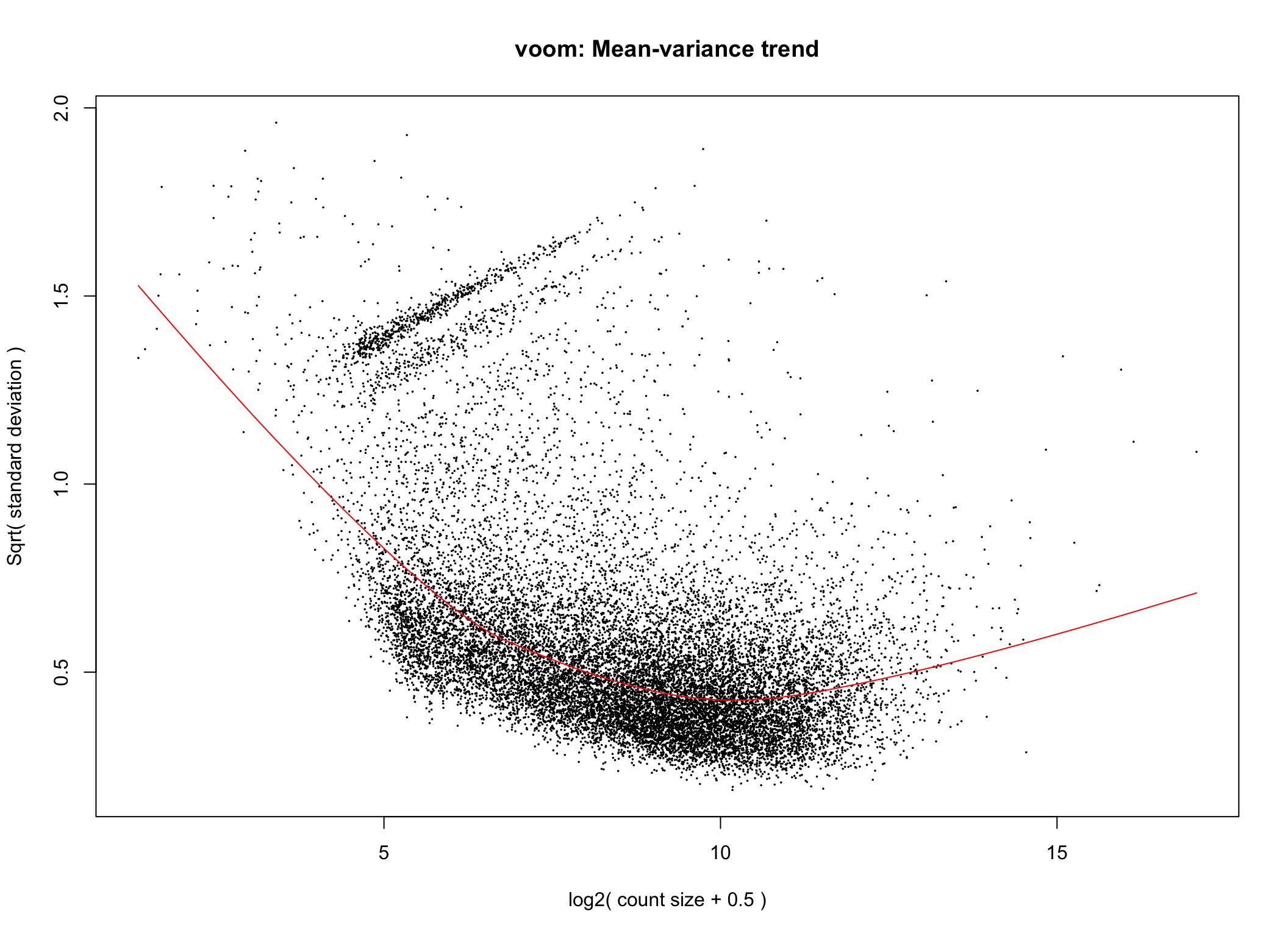

Voom transformation with observational weights

Version	Author	Date
d71eeb4	Ha Tran	2024-10-16
ae93fcc	tranmanhha135	2024-02-02
2c24612	tranmanhha135	2022-10-13
959a5df	tranmanhha135	2022-09-07
f4ba25b	Ha Manh Tran	2021-11-23

Observational and group level weights

# voom transformation with sample weights using full_design matrix for group-specific weights
voom1 <- limma::voomWithQualityWeights(counts = dge, design = full_design, plot = TRUE)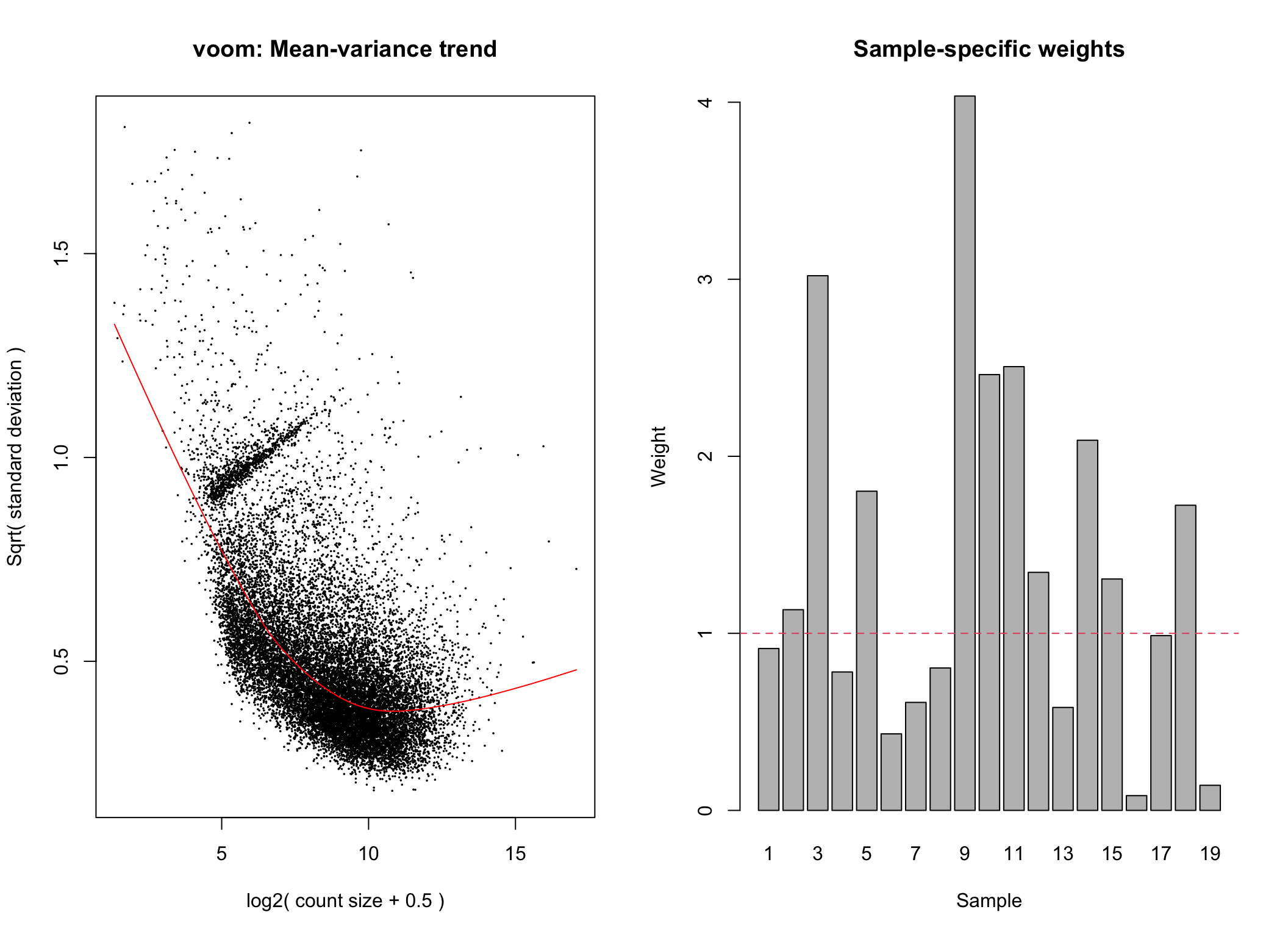

Voom transformation with observational and group-specific weights

Version	Author	Date
d71eeb4	Ha Tran	2024-10-16
ae93fcc	tranmanhha135	2024-02-02
2c24612	tranmanhha135	2022-10-13
959a5df	tranmanhha135	2022-09-07

Observational and sample level weights

# voom transformation with sample weights using null design matrix
voom2 <- limma::voomWithQualityWeights(counts = dge,design = null_design, plot = TRUE)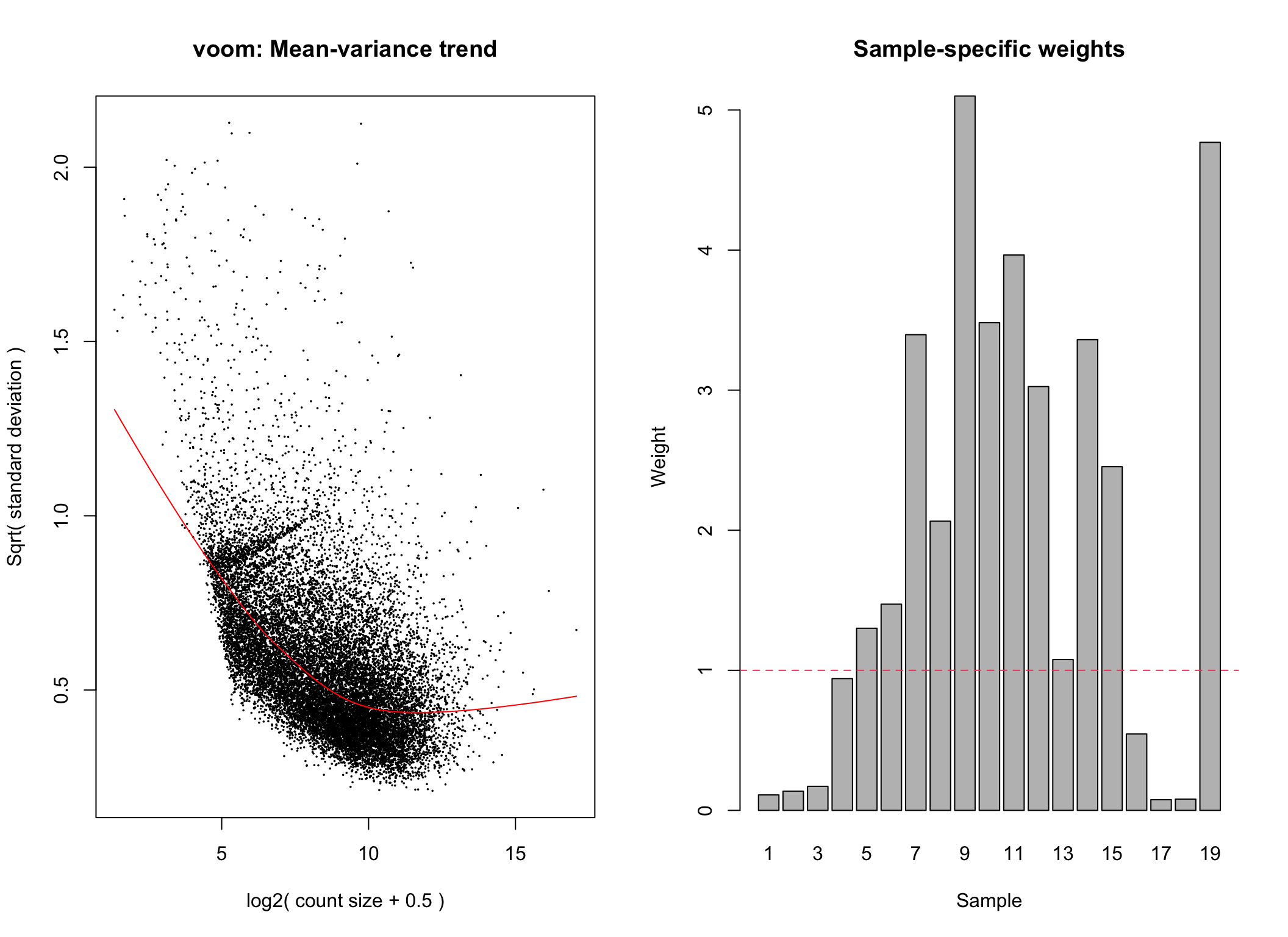

Voom transformation with observational and sample-specific weights

Version	Author	Date
d71eeb4	Ha Tran	2024-10-16
ae93fcc	tranmanhha135	2024-02-02
2c24612	tranmanhha135	2022-10-13
959a5df	tranmanhha135	2022-09-07

Visualisation of Voom transformation

Groups and sample weights

Equal quality samples should ideally receive a weight of 1. When weights are calculated across all samples irrespective of their groups, the two extreme VAS groups have reduced weights

# function for extracting weights from voom transformation and generating a bar plot
lapply(1:2, function(num){
  
  name <-  get(paste0('voom',num))
  name$targets %>% 
    rownames_to_column("Sample") %>% 
    as_tibble() %>% 
    ggplot(aes(x = Sample, y = sample.weights, fill = group)) +
    scale_fill_manual(values = groupColour) +
    geom_bar(stat = "identity", alpha = 0.8) +
    labs(x = "", y = "Sample Weights", fill = "") +
    geom_hline(yintercept = 1) +
    bossTheme()+
    theme(axis.text.x = element_text(angle = 90, hjust = 1, vjust = 0.5))
  
}) %>% patch(., legend = "right") %>% patch_ymax()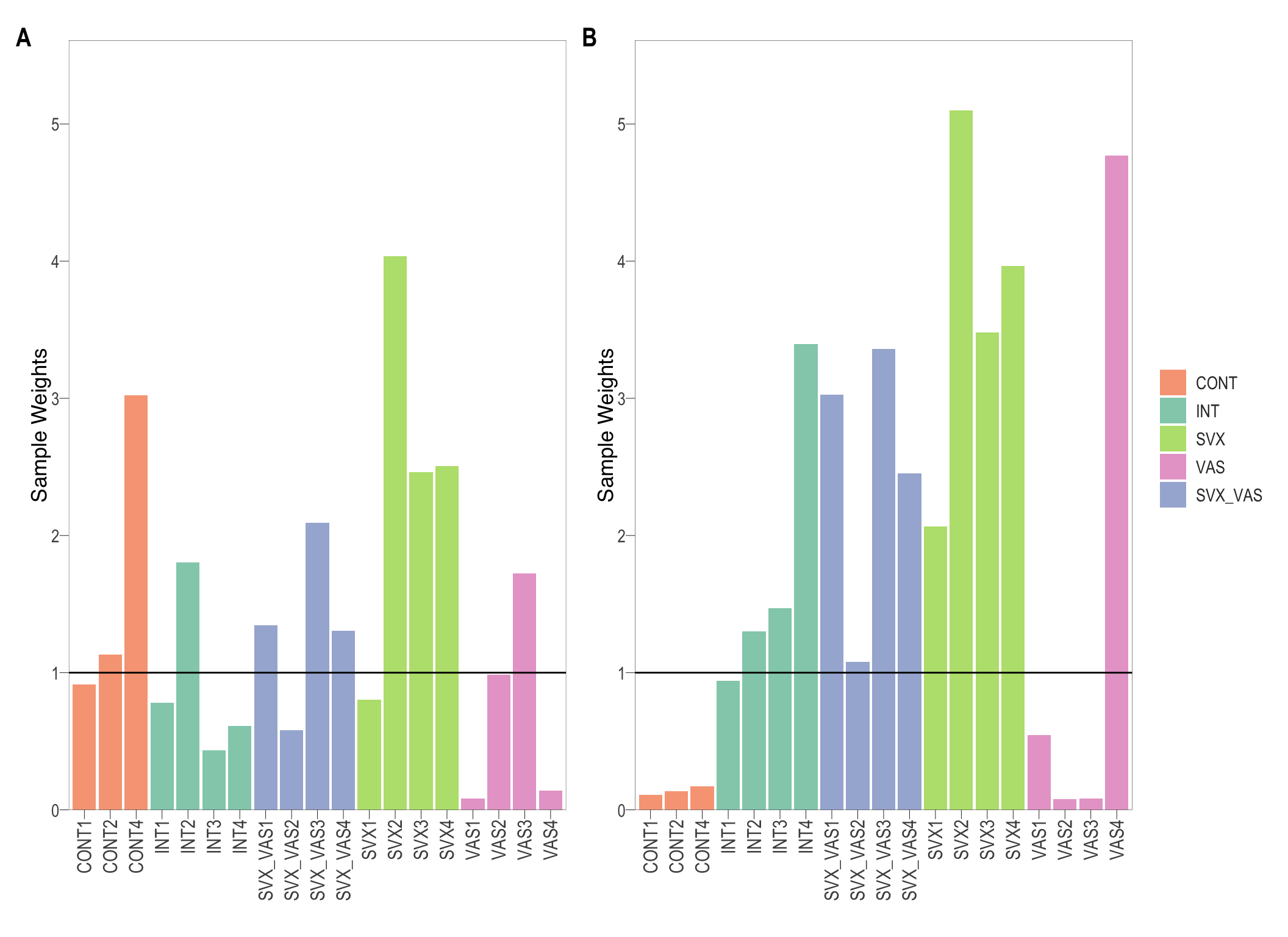

Group and samples specific weights

Version	Author	Date
d71eeb4	Ha Tran	2024-10-16
ae93fcc	tranmanhha135	2024-02-02
2c24612	tranmanhha135	2022-10-13
959a5df	tranmanhha135	2022-09-07

PCA

After the voom transformation, another PCA plot can be generated. This time the sample weights are represented by size.

# Function for performing pca and generating plots
voom_pca <- function(voom_trans, titleIndex){
  title <- c("Group-level weights", "Sample-level weights")
  pca <- voom_trans$E %>% 
    t() %>% 
    prcomp()
  
  voom_trans$targets <- voom_trans$targets %>% as.data.frame %>% rownames_to_column("Sample_Name")

  pca$x %>%
    as.data.frame() %>%
    rownames_to_column("Sample_Name") %>%
    as_tibble() %>%
    dplyr::select(Sample_Name, PC1, PC2) %>%
    left_join(voom_trans$targets, by = "Sample_Name") %>%
    mutate(sample.weights = round(sample.weights, 3)) %>%
    ggplot(aes(PC1, PC2, colour = group, size = sample.weights, label = Sample_Name)) +
    geom_label_repel(box.padding = grid::unit(0.5,"lines"), size = 3, label.size = 0.15, show.legend = F) +
    geom_point(alpha = 0.5) +
    scale_color_manual(values = groupColour_dark) +
    scale_size_continuous(limits=c(0,5)) +
    labs(x = paste0("PC1 (", percent(summary(pca)$importance["Proportion of Variance","PC1"]),")"),
         y = paste0("PC2 (", percent(summary(pca)$importance["Proportion of Variance","PC2"]),")"),
         colour = "",
         size = "Weights",
         title = title[titleIndex %>% as.numeric()]) +
    bossTheme(legend = "bottom") +
    
    guides(colour = guide_legend(override.aes = list(size = 3)))
}

# iterate with lapply for voom 1 and 2
 lapply(c("1","2"), function(y){
  voom_pca(voom_trans = get(paste0('voom',y)), titleIndex = y)
}) %>% patch(., legend = "bottom")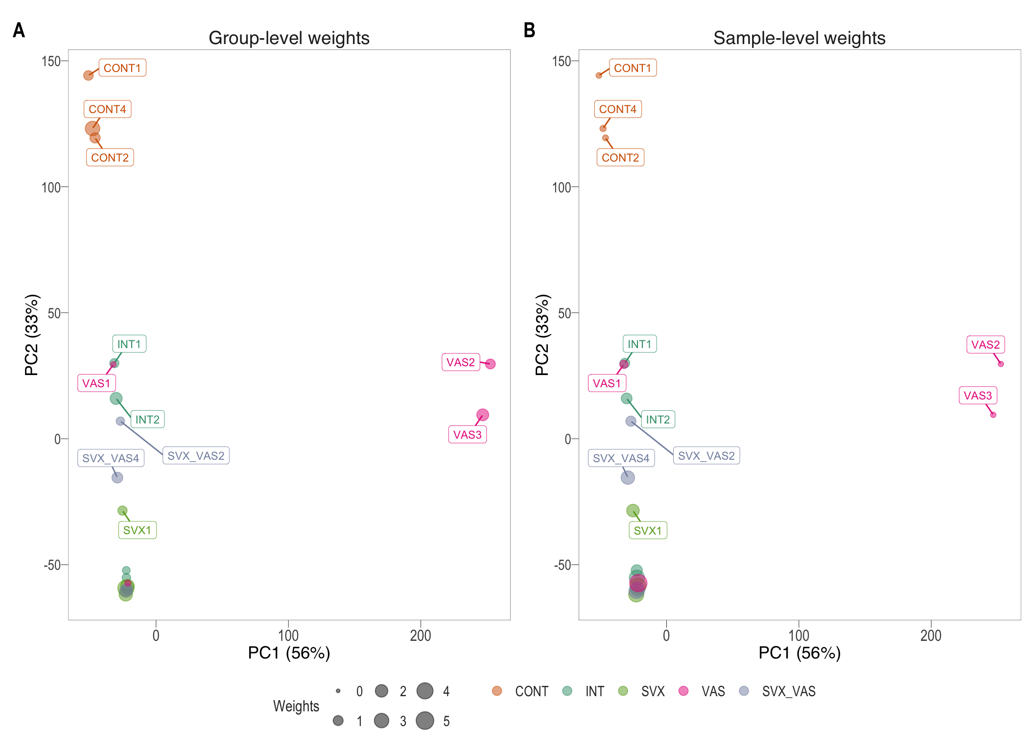

PCA plots after voom quality weight transformations. Group-specific weights(left) and sample-specific weights (right)

Version	Author	Date
d71eeb4	Ha Tran	2024-10-16
ae93fcc	tranmanhha135	2024-02-02
2c24612	tranmanhha135	2022-10-13
959a5df	tranmanhha135	2022-09-07

PC1 increased and PC2 decreased slightly from the previous PCA plot. The clustering of do not appear to signficantly change, however, the addition of sample weights should give a better fit for linear model. Following voom transformation, the observational and sample-specific weights are used to fit the linear model and

Apply linear model

Without FC cutoff using TREAT After playing around with the P value adjustment method and the p.value/adj.p.Value cutoff. The DE analysis of sample-weighted data at an un-adjusted P value of 0.01 generated the most favorable number of DE genes (Table 1). Adjustment of p-value through any method removes majority of DE genes from most comparison, even when the adjustment method is relatively relaxed (e.g. FDR and BH).

With FC cutoff using TREAT However, without FC cutoff and p-value of 0.01, the INT vs CONT comparison still have over 8000 DE genes. Thus, we can afford to be more stringent with our adjustment method and adj.p.val cutoff. Additionally, when the list of DE genes is large, we can apply a fold change cutoff through application of TREAT to prioritise the genes with greater fold changes and potentially more biologically relevant. Idealy, we are aiming for ~300 genes genes. IPA analysis with this number of genes should generate meaningful results.

Importantly, the FC threshold used in TREAT should be chosen as a small value below which results should be ignored, instead of a target fold-change. In general, a modest fold-change of 1.1 - 1.5 is recommended. However, it is more important to select a fold-change cutoff that generates a sufficiently small list of DE genes.

A fold-change value of 1.5 and FDR<0.05, generated a sufficiently small number of DE genes for the INT vs CONT comparison. This should be sufficient for functional enrichment analysis (Table 12).

# specifying FC of interest
options(digits = 6)
fc <- c("none", 1.1, 1.2, 1.5)

FC=none

# function for applying linear model, generate decideTest table, and extract topTable
limmaFit <- function(x, fc, adjMethod, p.val, tableNum, list = F){
  lm <- limma::lmFit(object = x, design = full_design) %>%
    contrasts.fit(contrasts = contrast)
  
  if (fc == "none") {
    lm <- lm %>% limma::eBayes()
  } else {
    lm <- lm %>% limma::treat(fc = as.numeric(fc))
  }
  
  
  if (list == TRUE) { 
    
    if (fc == "none") {
      lm_all <- lapply(1:ncol(lm), function(y){
        limma::topTable(lm, coef = y, number = Inf, adjust.method = adjMethod)
      })
    } else {
      lm_all <- lapply(1:ncol(lm), function(y){
        limma::topTreat(lm, coef = y, number = Inf, adjust.method = adjMethod) 
      })
    }
    
    lapply(lm_all, function(x) {
      df <- x %>% as.data.frame() %>% 
        dplyr::mutate(expression = case_when(
          adj.P.Val <= p.val & logFC >=0 ~ "up",
          adj.P.Val <= p.val & logFC <0 ~ "down",
          TRUE ~ "insig"))
      
      df$expression <- factor(df$expression, levels = c("insig", "down", "up"))
      # df$entrezid <- df$entrezid %>% as.character()
      
      return(df)
      
    })
    
  } else {
    
    lm_dt <- decideTests(object = lm, adjust.method = adjMethod, p.value = p.val)
    print(knitr::kable(summary(lm_dt)
                       , caption = paste0("TABLE ",tableNum, ": Number of significant DE genes from '", deparse(substitute(x)), "' with '", adjMethod, "' adjusment method, and at a p-value/adj.p-value of ", p.val)) %>% 
            kable_styling(bootstrap_options = c("striped", "hover")))
    
  }
}

limmaFit(x = voom2, fc[1], adjMethod = "none", p.val = 0.01, 1)

TABLE 1: Number of significant DE genes from ‘voom2’ with ‘none’ adjusment method, and at a p-value/adj.p-value of 0.01
	INT vs CONT	INT vs SVX_VAS	SVX vs SVX_VAS	VAS vs SVX_VAS	SVX_VAS vs CONT	INT vs VAS
Down	305	98	81	96	494	58
NotSig	14943	16988	17028	16987	14566	17116
Up	1974	136	113	139	2162	48

limmaFit(x = voom2, fc[1], adjMethod = "fdr", p.val = 0.1, 2)

TABLE 2: Number of significant DE genes from ‘voom2’ with ‘fdr’ adjusment method, and at a p-value/adj.p-value of 0.1
	INT vs CONT	INT vs SVX_VAS	SVX vs SVX_VAS	VAS vs SVX_VAS	SVX_VAS vs CONT	INT vs VAS
Down	510	5	0	0	1021	0
NotSig	14423	17213	17222	17220	13522	17222
Up	2289	4	0	2	2679	0

limmaFit(x = voom2, fc[1], adjMethod = "fdr", p.val = 0.05, 3)

TABLE 3: Number of significant DE genes from ‘voom2’ with ‘fdr’ adjusment method, and at a p-value/adj.p-value of 0.05
	INT vs CONT	INT vs SVX_VAS	SVX vs SVX_VAS	VAS vs SVX_VAS	SVX_VAS vs CONT	INT vs VAS
Down	134	0	0	0	328	0
NotSig	15484	17221	17222	17220	15001	17222
Up	1604	1	0	2	1893	0

FC=1.1

limmaFit(x = voom2, fc[2], adjMethod = "none", p.val = 0.01,4)

TABLE 4: Number of significant DE genes from ‘voom2’ with ‘none’ adjusment method, and at a p-value/adj.p-value of 0.01
	INT vs CONT	INT vs SVX_VAS	SVX vs SVX_VAS	VAS vs SVX_VAS	SVX_VAS vs CONT	INT vs VAS
Down	187	40	10	24	344	13
NotSig	15205	17126	17188	17140	14883	17200
Up	1830	56	24	58	1995	9

limmaFit(x = voom2, fc[2], adjMethod = "fdr", p.val = 0.1, 5)

TABLE 5: Number of significant DE genes from ‘voom2’ with ‘fdr’ adjusment method, and at a p-value/adj.p-value of 0.1
	INT vs CONT	INT vs SVX_VAS	SVX vs SVX_VAS	VAS vs SVX_VAS	SVX_VAS vs CONT	INT vs VAS
Down	253	0	0	0	601	0
NotSig	15006	17222	17222	17222	14292	17222
Up	1963	0	0	0	2329	0

limmaFit(x = voom2, fc[2], adjMethod = "fdr", p.val = 0.05, 6)

TABLE 6: Number of significant DE genes from ‘voom2’ with ‘fdr’ adjusment method, and at a p-value/adj.p-value of 0.05
	INT vs CONT	INT vs SVX_VAS	SVX vs SVX_VAS	VAS vs SVX_VAS	SVX_VAS vs CONT	INT vs VAS
Down	55	0	0	0	151	0
NotSig	15775	17222	17222	17222	15430	17222
Up	1392	0	0	0	1641	0

FC=1.2

limmaFit(x = voom2, fc[3], adjMethod = "none", p.val = 0.01,7)

TABLE 7: Number of significant DE genes from ‘voom2’ with ‘none’ adjusment method, and at a p-value/adj.p-value of 0.01
	INT vs CONT	INT vs SVX_VAS	SVX vs SVX_VAS	VAS vs SVX_VAS	SVX_VAS vs CONT	INT vs VAS
Down	80	13	3	10	165	4
NotSig	15558	17191	17215	17183	15320	17213
Up	1584	18	4	29	1737	5

limmaFit(x = voom2, fc[3], adjMethod = "fdr", p.val = 0.1, 8)

TABLE 8: Number of significant DE genes from ‘voom2’ with ‘fdr’ adjusment method, and at a p-value/adj.p-value of 0.1
	INT vs CONT	INT vs SVX_VAS	SVX vs SVX_VAS	VAS vs SVX_VAS	SVX_VAS vs CONT	INT vs VAS
Down	74	0	0	0	202	0
NotSig	15588	17222	17222	17222	15199	17222
Up	1560	0	0	0	1821	0

limmaFit(x = voom2, fc[3], adjMethod = "fdr", p.val = 0.05, 9)

TABLE 9: Number of significant DE genes from ‘voom2’ with ‘fdr’ adjusment method, and at a p-value/adj.p-value of 0.05
	INT vs CONT	INT vs SVX_VAS	SVX vs SVX_VAS	VAS vs SVX_VAS	SVX_VAS vs CONT	INT vs VAS
Down	15	0	0	0	47	0
NotSig	16161	17222	17222	17222	15924	17222
Up	1046	0	0	0	1251	0

FC=1.5

limmaFit(x = voom2, fc[4], adjMethod = "none", p.val = 0.01,10)

TABLE 10: Number of significant DE genes from ‘voom2’ with ‘none’ adjusment method, and at a p-value/adj.p-value of 0.01
	INT vs CONT	INT vs SVX_VAS	SVX vs SVX_VAS	VAS vs SVX_VAS	SVX_VAS vs CONT	INT vs VAS
Down	14	1	0	2	29	0
NotSig	16238	17216	17222	17214	16132	17220
Up	970	5	0	6	1061	2

limmaFit(x = voom2, fc[4], adjMethod = "fdr", p.val = 0.1, 11)

TABLE 11: Number of significant DE genes from ‘voom2’ with ‘fdr’ adjusment method, and at a p-value/adj.p-value of 0.1
	INT vs CONT	INT vs SVX_VAS	SVX vs SVX_VAS	VAS vs SVX_VAS	SVX_VAS vs CONT	INT vs VAS
Down	6	0	0	0	14	0
NotSig	16542	17222	17222	17222	16385	17222
Up	674	0	0	0	823	0

limmaFit(x = voom2, fc[4], adjMethod = "fdr", p.val = 0.05, 12)

TABLE 12: Number of significant DE genes from ‘voom2’ with ‘fdr’ adjusment method, and at a p-value/adj.p-value of 0.05
	INT vs CONT	INT vs SVX_VAS	SVX vs SVX_VAS	VAS vs SVX_VAS	SVX_VAS vs CONT	INT vs VAS
Down	2	0	0	0	5	0
NotSig	16834	17222	17222	17222	16712	17222
Up	386	0	0	0	505	0

Differential Gene Expression analysis

For the first Intact vs Control comparison, a rigorous statistical test was used to reduce the list of DE genes down to a more biologically relevant number. This included testing significance relative to a fold change threshold (TREAT). For this comparison, genes significantly above of FC of 1.5 and FDR < 0.05 are visualised.

For the other comparisons (Intact vs SVX_VAS, SVX vs SVX_VAS, and VAS vs SVX_VAS), a less stringent test was applied to identify significant DE genes while maintaining sufficient number of downstream functional enrichment analysis. Genes with P.value < 0.01 are visualised as follows:

P-value histogram: illustrates the distribution of p-values. As the stringency increases (increasing FC threshold), the distribution shifts towards 1, thus insignificant.
MA plot: helps visualise and identify genes with significant changes in expression. Points deviating from the central axis often indicate differentially expressed genes, allowing assessment of the magnitude and consistency of expression changes across conditions.
- \(x-axis =\) average expression, in log counts per million (CPM)
- \(y-axis =\) log fold change between conditions
Volcano plot: shows significantly differentially expressed genes appearing as points that are both statistically significant (located at the top) and have substantial fold changes (located on the left or right sides). This visualization enables identification of genes that are statistically and biologically significant.
- \(x-axis =\) log fold change between conditions
- \(y-axis =\) negative logarithm of the FDR-adjusted p-values
Heatmap: visualize gene expression patterns across different experimental conditions. Rows are genes, columns represent samples, and the colour intensity indicates the expression level of a gene in a specific sample. The genes are also clustered based on similar expression patterns, which provides insights into the overall structure and relationships within large datasets.
- These heatmaps illustrates the top 30 most significant DE genes
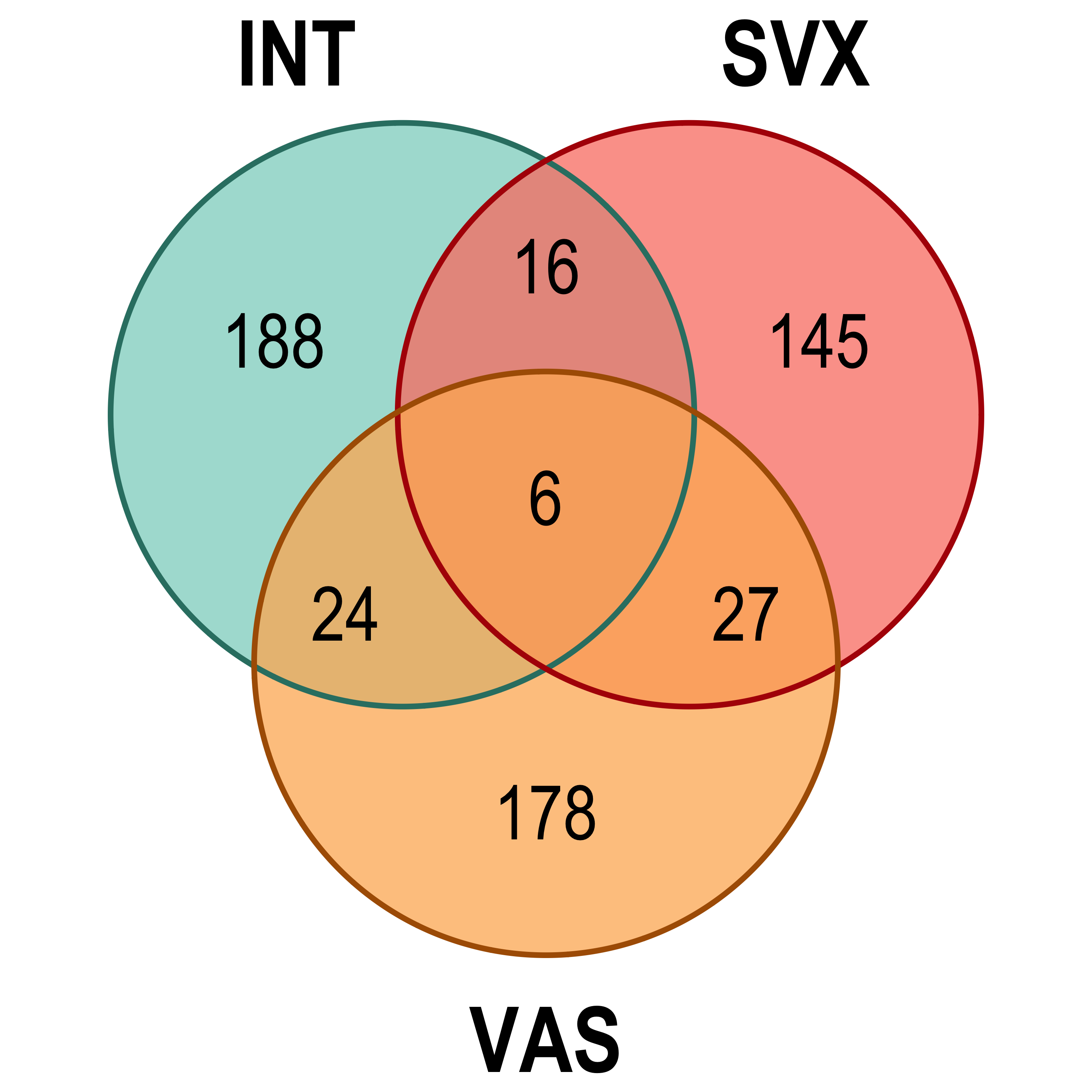
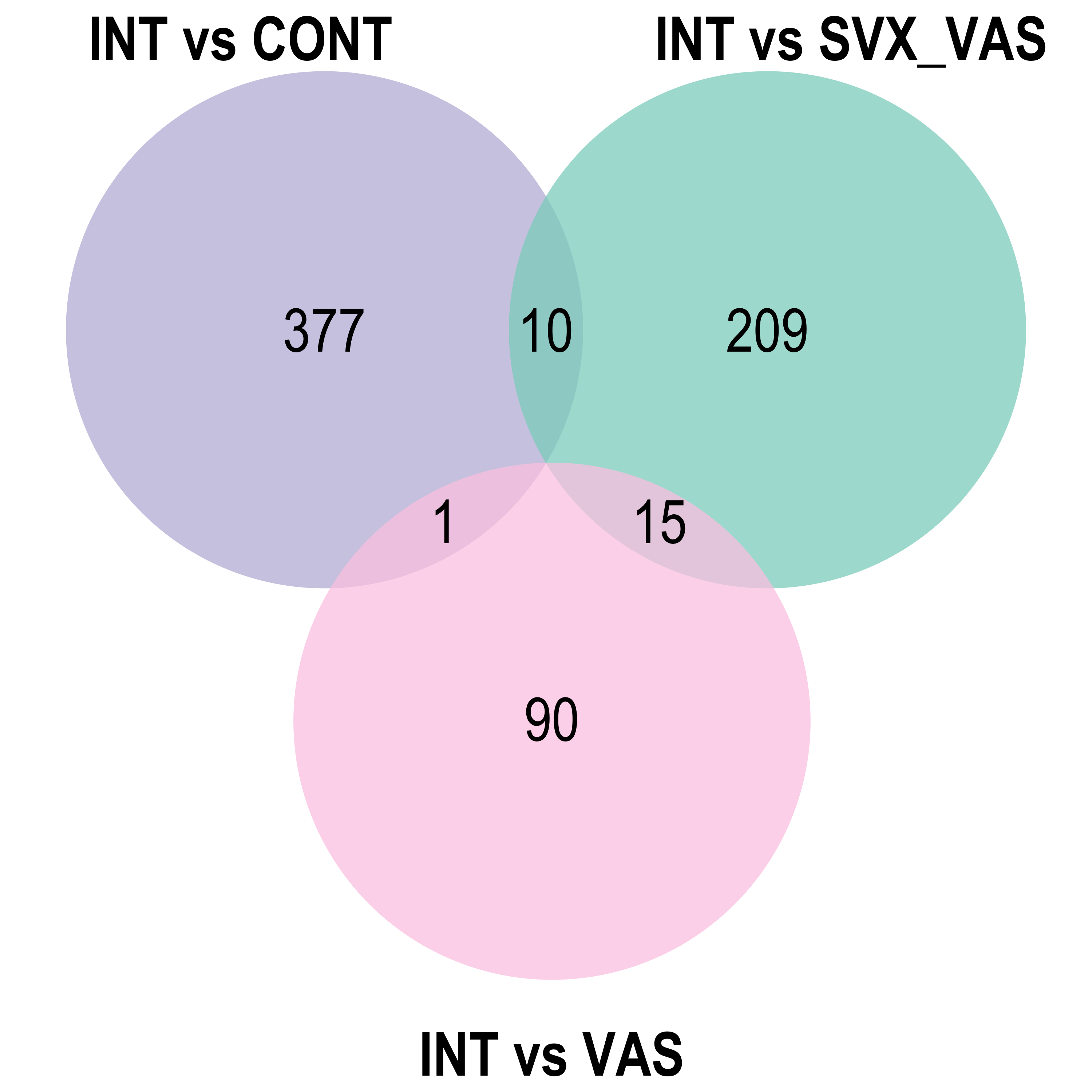
Venn diagram: visualises the significant DE gene overlap between the previous RNA-seq experiment and the current.

comp <- colnames(contrast)


options(digits = 6)

# High stringency for the first comparison
highStringency <- limmaFit(x = voom2, fc = 1.5, adjMethod = "fdr", p.val = 0.05, list = T)
highStringency_sig <- lapply(1:ncol(contrast), function(i){filter(highStringency[[i]], adj.P.Val < 0.05)})

# Low stringency for the other three comparison
lowStringency <- limmaFit(x = voom2, fc = "none", adjMethod = "none", p.val = 0.01, list = T)
lowStringency_sig <- lapply(1:ncol(contrast), function(i){filter(lowStringency[[i]], adj.P.Val < 0.01)})

lm_all <- list(highStringency[[1]], lowStringency[[2]], lowStringency[[3]], lowStringency[[4]], highStringency[[5]], lowStringency[[6]]) %>% setNames(colnames(contrast))

lm_sig <- list(highStringency_sig[[1]], lowStringency_sig[[2]], lowStringency_sig[[3]], lowStringency_sig[[4]], highStringency_sig[[5]],lowStringency_sig[[6]]) %>% setNames(colnames(contrast))

INT vs CONT

P-val histogram

lm_hist <- list()
for (name in comp) {
  lm_hist[[name]] <- ggplot(lm_all[[name]] %>% as.data.frame(), aes(x = P.Value)) +
    geom_histogram(bins = 50, fill="#8DA0CB",colour= "white", linewidth = 0.2, alpha=0.9) +
    scale_y_continuous(expand = expansion(mult = c(0, .1))) +
    labs(x = "P values", y = "Counts") +
    bossTheme()
  
  if (savePlots == T) {
    ggsave(paste0("hist_",name,".svg"),
           plot = lm_hist[[name]],
           path = here::here("2_plots/2_DE/"),
           width = 13,
           height = 11,
           units = "cm")
  }
}

lm_hist[[1]]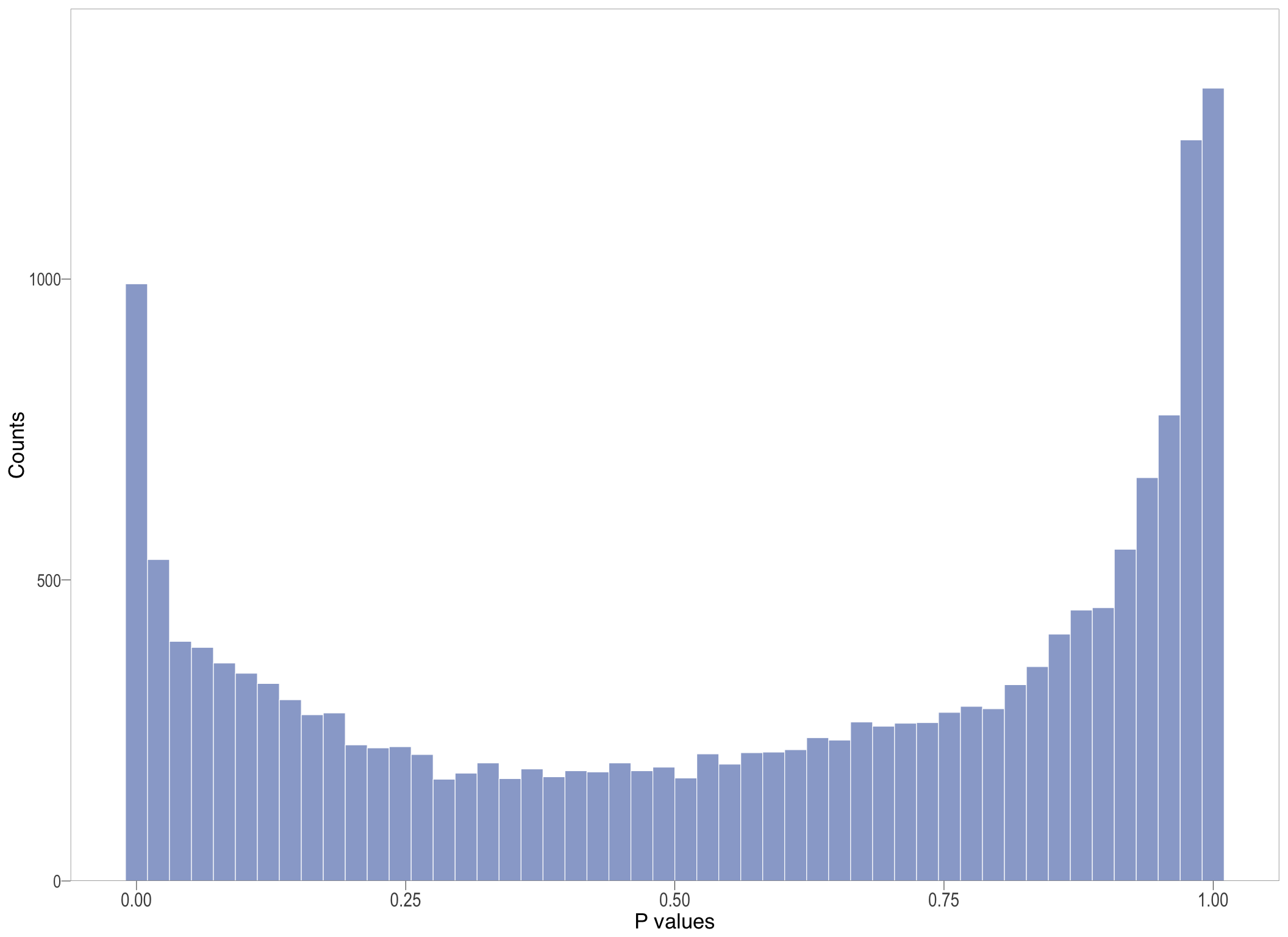

Version	Author	Date
d71eeb4	Ha Tran	2024-10-16

MA plot

ma <- list()
for (name in comp) {
  top <- 5
  top_limma <- bind_rows(
    lm_all[[name]] %>%
      dplyr::filter(expression == "up") %>%
      arrange(adj.P.Val, desc(abs(logFC))) %>%
      head(top),
    lm_all[[name]] %>%
      dplyr::filter(expression == "down") %>%
      arrange(adj.P.Val, desc(abs(logFC))) %>%
      head(top)
  )
  invisible(top_limma %>% as.data.frame())
  
  max <- max(lm_all[[name]]$logFC)

  ma[[name]] <- lm_all[[name]] %>% dplyr::arrange(expression) %>% 
    ggplot(aes(x = AveExpr, y = logFC)) +
    geom_point(aes(colour = expression, size = expression),show.legend = T, alpha = 0.7, stroke =0) +
    geom_label_repel(data = top_limma, # map labels, visit ?geom_label_repel
                     mapping = aes(label = gene_name),
                     size = 3,
                     label.padding = 0.15,
                     label.size = 0,
                     label.r = 0.15,
                     box.padding = 0.9,
                     point.padding = 0.5,
                     segment.size = 0.3,
                     segment.color = "grey50"
                     ) +
    labs(
      x = expression("log"[2] * "CPM"),
      y = expression("log"[2] * "FC"),
      colour = "Expression") + 
    geom_hline(yintercept = 0, linetype = "dashed") +
    scale_y_continuous(limits = c(-max,max), expand = expansion(mult = c(0.05, 0.05))) +
    scale_size_manual(values = c(1.5,2.4,2.4), guide = "none") +
    scale_fill_manual(values = expressionCol) +
    scale_color_manual(labels = c(paste0("NS: ", sum(lm_all[[name]]$expression == "insig"), "  "),
                                  paste0("Down: ", sum(lm_all[[name]]$expression == "down"), "  "),
                                  paste0("Up: ", sum(lm_all[[name]]$expression == "up"), " ")), 
                       values = expressionCol_dark) +    
    bossTheme(base_size = 14, legend = "bottom") +
    guides(colour = guide_legend(override.aes = list(size = 2.4)))
  
  
  if (savePlots) {
    ggsave(paste0("ma_", name, ".png"),
           plot = ma[[name]],
           path = here::here("2_plots/2_DE/"),
           width = 13,
           height = 11,
           units = "cm",
           dpi = 900)
  }
  
}

saveRDS(ma, here::here("0_data/RDS_plots/ma_plots.rds"))

# display
ma[[1]]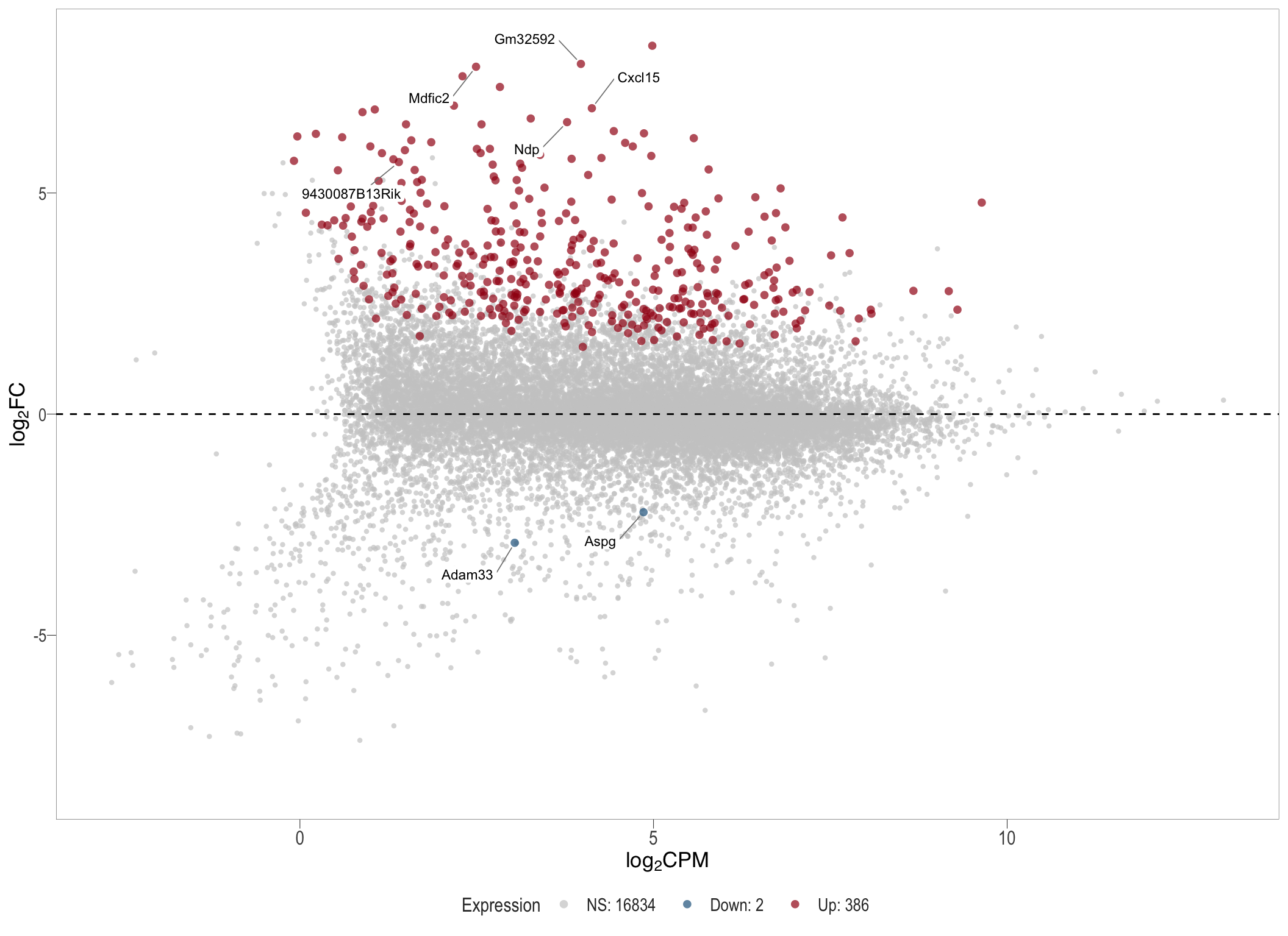

Version	Author	Date
d71eeb4	Ha Tran	2024-10-16
ae93fcc	tranmanhha135	2024-02-02
2c24612	tranmanhha135	2022-10-13
1101367	tranmanhha135	2022-10-02
192d010	tranmanhha135	2022-09-20
959a5df	tranmanhha135	2022-09-07
32454d5	Ha Manh Tran	2022-01-01
3b268fc	Ha Tran	2021-12-09

Volcano plot

library(ggrastr)
vol <- list()
for (name in comp) {
    top <- 5
    top_limma <- bind_rows(
      lm_all[[name]] %>%
        dplyr::filter(expression == "up") %>%
        arrange(adj.P.Val, desc(abs(logFC))) %>%
        head(top),
      lm_all[[name]] %>%
        dplyr::filter(expression == "down") %>%
        arrange(adj.P.Val, desc(abs(logFC))) %>%
        head(top)
    )
    invisible(top_limma %>% as.data.frame())
    max <- max(lm_all[[name]]$logFC)
    vol[[name]] <- lm_all[[name]] %>%
      ggplot(aes(x = logFC,y = -log(adj.P.Val, 10))) +
      rasterise(geom_point(aes(colour = expression, size = expression), show.legend = T, alpha =0.7, stroke =0 ), dpi = 600) +
      geom_label_repel(data = top_limma,
                         # lm_all[[name]] %>% dplyr::filter(gene_name %in% c("Itprid1", "Scart1", "Blk", "Cd3e", "Trgc1", "Il7r","Nr4a3","Coch")), 
                       mapping = aes(label = gene_name),
                       size = 5,
                       label.padding = 0.15,
                       label.size = 0,
                       label.r = 0.15,
                       box.padding = 0.9,
                       point.padding = 0.5,
                       segment.size = 0.3,
                       segment.color = "grey50") +
      labs(x = expression("log"[2] * "FC"),
           y = expression("-log"[10] * "FDR"),
           colour = "Expression") +
      scale_x_continuous(limits = c(-max,max),expand = expansion(mult = c(0.01, 0.01))) +
      scale_size_manual(values = c(1.5,2.4,2.4), guide = "none") +
      scale_fill_manual(values = expressionCol) +
      scale_color_manual(labels = c(paste0("NS: ", sum(lm_all[[name]]$expression == "insig"), "  "),
                                    paste0("Down: ", sum(lm_all[[name]]$expression == "down"), "  "),
                                    paste0("Up: ", sum(lm_all[[name]]$expression == "up"), " ")), 
                         values = expressionCol_dark) +    
      bossTheme( legend = "bottom") +
      guides(colour = guide_legend(override.aes = list(size = 2.4)))
    
    
    if (savePlots == T) { 
      ggsave(paste0("vol_", name, ".png"),
             plot = vol[[name]],
             path = here::here("2_plots/2_DE/"),
             width = 11,
             height = 13,
             units = "cm",
             dpi = 900)
    }
  
}

saveRDS(vol, here::here("0_data/RDS_plots/vol_plots.rds"))

# display
vol[[1]]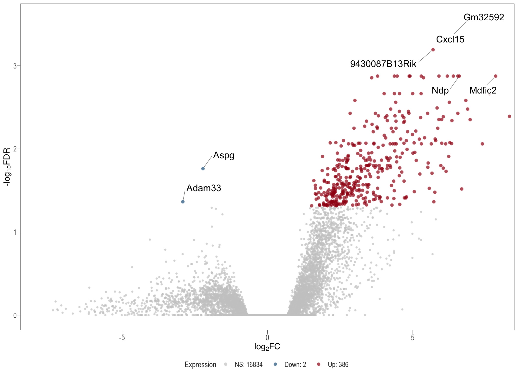

Version	Author	Date
d519e7f	Ha Tran	2024-12-03
d71eeb4	Ha Tran	2024-10-16
ae93fcc	tranmanhha135	2024-02-02
2c24612	tranmanhha135	2022-10-13
1101367	tranmanhha135	2022-10-02
192d010	tranmanhha135	2022-09-20
959a5df	tranmanhha135	2022-09-07
32454d5	Ha Manh Tran	2022-01-01
3b268fc	Ha Tran	2021-12-09

ggsave(filename = "intVsvxVAS.svg", plot = vol[[2]],path = here::here("2_plots/"), width = 12, height = 12, units = "cm")

Top upregulated

logCPM_up=list()
logCPM_down=list()
anno=list()
anno_colours=list()

for (i in 1:length(comp)) {
  x <- comp[i] %>% as.character()
  
  # initialise/reinitialise the count matrix
  logCPM <- cpm(dge, prior.count = 3, log = TRUE) 
  rownames(logCPM) <- dge$genes$gene_name
  colnames(logCPM) <- dge$samples$pretty
  
  # initialise/reinitialise the annotations used for heatmap legend
  anno[[x]] <- as.factor(dge$samples$group) %>% as.data.frame()
  colnames(anno[[x]]) <- "Groups"

  
  if (i == 1) { # for the first comparison, extract just intact and control
    logCPM <- subset(logCPM ,select = 1:7)
    anno[[x]] <- dplyr::slice(anno[[x]], 1:7)
    rownames(anno[[x]]) <- colnames(logCPM) } 
  if (i == 2) { # for the second comapsion, extract intact and SVX_VAS
    logCPM <- subset(logCPM, select = c(4:7,12:15))
    anno[[x]] <- dplyr::slice(anno[[x]], c(4:7,12:15))
    rownames(anno[[x]]) <- colnames(logCPM) } 
  if (i == 3) { # for the second comapsion, extract SVX and SVX_VAS
    logCPM <- subset(logCPM, select = 8:15)
    anno[[x]] <- dplyr::slice(anno[[x]], 8:15)
    rownames(anno[[x]]) <- colnames(logCPM) } 
  if (i == 4) { # for the second comapsion, extract VAS and SVX_VAS
    logCPM <- subset(logCPM, select = c(16:19, 12:15))
    anno[[x]] <- dplyr::slice(anno[[x]], c(16:19, 12:15))
    rownames(anno[[x]]) <- colnames(logCPM) }
  if (i == 5) { # for the first comparison, extract just intact and control
    logCPM <- subset(logCPM ,select = c(12:15,1:3))
    anno[[x]] <- dplyr::slice(anno[[x]], c(12:15,1:3))
    rownames(anno[[x]]) <- colnames(logCPM) } 
  if (i == 6) { # for the first comparison, extract just intact and control
    logCPM <- subset(logCPM ,select = c(4:7,16:19))
    anno[[x]] <- dplyr::slice(anno[[x]], c(4:7,16:19))
    rownames(anno[[x]]) <- colnames(logCPM) } 
  
  # filtering top unregulated genes then filter the logCPM values of those genes.
  upReg <- lm_sig[[x]] %>%
    dplyr::filter(logFC > 0) %>%
    arrange(sort(adj.P.Val, decreasing = F))
  upReg <- upReg[1:20,]
  logCPM_up[[x]] <- logCPM[upReg$gene_name,] %>% as.data.frame()
  
  # filtering top unregulated genes then filter the logCPM values of those genes.
  downReg <- lm_sig[[x]] %>%
    dplyr::filter(logFC < 0) %>%
    arrange(sort(adj.P.Val, decreasing = F))
  if (nrow(downReg) >= 20) {max <-  20} else {max <-  nrow(downReg)}
  downReg <- downReg[1:max,] %>% na.omit()
  logCPM_down[[x]] <- logCPM[downReg$gene_name,] %>% na.omit %>%  as.data.frame()
}

library(ggplotify)
heat_up=list()

custom_heatUp <- function(direction, ...){
  
  if (direction == "up") {
    mat <- logCPM_up[[x]]
  } else {
    mat <- logCPM_down[[x]]
  }
  
  ComplexHeatmap::pheatmap(
    mat = mat, 
    color = colorRampPalette(rev(c("#FB8072","#FDB462","#ffffd5","#8DD3C7","#80B1D3")))(100),
    # cellheight = 20,
    cellwidth = 30,
    scale = "row",
    border_color = "white",
    treeheight_row = 40,
    treeheight_col = 30,
    show_colnames = T,
    clustering_distance_rows = "euclidean",
    main = paste0("Top ", nrow(mat), " significant ", direction,"regulated genes\n"),

    legend = F,

    # heatmap_legend_param = list(title = "Z-score",
    #                             legend_direction = "vertical",
    #                             legend_width = unit(5, "cm")),

    # annotation = T,
    annotation_legend = T,
    annotation_col = anno[[x]],
    annotation_colors = list("Groups" = groupColour),
    annotation_names_col = F,

    fontfamily = "Arial Narrow",
    fontsize = 14,
    fontsize_col = 14,
    fontsize_number = 14,
    fontsize_row = 14,
    labels_row = as.expression(lapply(rownames(mat), function(a) bquote(italic(.(a))))),
    ...) %>% as.ggplot()
}

for (i in 1:length(comp)) {
  x <- comp[i] %>% as.character()
  
  if (i == 1 || 5) {
    heat_up[[x]] <- custom_heatUp(direction = "up",
      cluster_cols = T,
      cutree_cols = 2,
      cutree_rows = 4
    )
  } else {
    heat_up[[x]] <- custom_heatUp(direction = "up",
      cluster_cols = T,
      cutree_cols = 2,
      cutree_rows = 4,
      # gaps_col = c(4)
    )
  }
  
  ggsave(paste0("heat_up_", comp[i], ".svg"),
         plot = heat_up[[x]],
         path = here::here("2_plots/2_DE/"),
         width = 166,
         height = 250,
         units = "mm"
  )
}

heat_up[[1]]

Version	Author	Date
d71eeb4	Ha Tran	2024-10-16
ae93fcc	tranmanhha135	2024-02-02
2c24612	tranmanhha135	2022-10-13
1101367	tranmanhha135	2022-10-02
959a5df	tranmanhha135	2022-09-07
32454d5	Ha Manh Tran	2022-01-01
3b268fc	Ha Tran	2021-12-09
f4ba25b	Ha Manh Tran	2021-11-23

Top downregulated

heat_down=list()

for (i in 1:length(comp)) {
  x <- comp[i] %>% as.character()
  
  if (i == 1 || 5) {
    heat_down[[x]] <- custom_heatUp(direction = "down",
      cluster_cols = T,
      cutree_cols = 2,
      cutree_rows = 2
    ) %>% as.ggplot()
  } else {
    heat_down[[x]] <- custom_heatUp(direction = "down",
      cluster_cols = T,
      cutree_cols = 2,
      cutree_rows = 4,
      # gaps_col = c(4)
    ) %>% as.ggplot()
  }
  
  ggsave(paste0("heat_down_", comp[i], ".svg"),
         plot = heat_down[[x]],
         path = here::here("2_plots/2_DE/"),
         width = 166,
         height = 250,
         units = "mm"
  )
}

heat_down[[1]]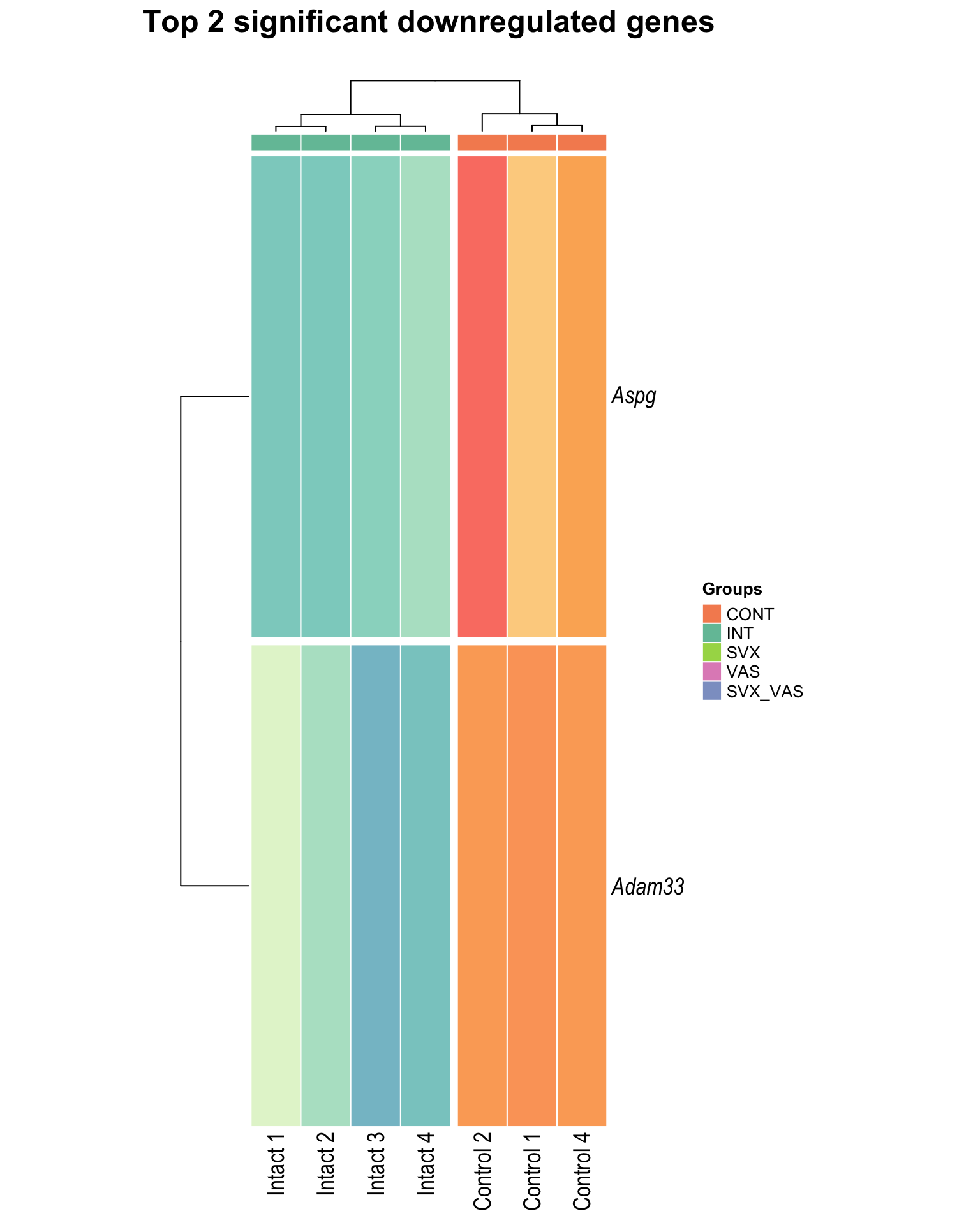

Version	Author	Date
d71eeb4	Ha Tran	2024-10-16
ae93fcc	tranmanhha135	2024-02-02
2c24612	tranmanhha135	2022-10-13
11a5cf4	tranmanhha135	2022-10-03
1101367	tranmanhha135	2022-10-02
192d010	tranmanhha135	2022-09-20
959a5df	tranmanhha135	2022-09-07
32454d5	Ha Manh Tran	2022-01-01
3b268fc	Ha Tran	2021-12-09
f4ba25b	Ha Manh Tran	2021-11-23

## this function is basically creating chunks within chunks, and then
## I use results='asis' so that the html image code is rendered 

library(knitr)

kexpand <- function(wd, ht, cap) {
  cat(knit(text = knit_expand(text = 
     sprintf("```{r %s, fig.width=%s, fig.height=%s}\n.pl\n```", cap,wd, ht)
)))}

# Loop through each FC value

types <- c("P-val histogram", "MA plot", "Volcano plot", "Top upregulated", "Top downregulated")

for (i in 2:length(comp)) {
  
  cat(paste0("## ",comp[i],"{.tabset .tabset-pills} \n\n"))

  cat(paste0("### ",types[[1]]," \n"))
  .pl <- lm_hist[[i]] 
  kexpand(wd = 10,ht = 6,cap = paste0("hist_",i))
  cat("\n\n")
  
  cat(paste0("### ",types[[2]]," \n"))
  .pl <- ma[[i]] 
  kexpand(wd = 10,ht = 6,cap = paste0("ma_",i))
  cat("\n\n")
  
  cat(paste0("### ",types[[3]]," \n"))
  .pl <- vol[[i]]
  kexpand(wd = 10,ht = 6,cap = paste0("vol_",i))
  cat("\n\n")
  
  cat(paste0("### ",types[[4]]," \n"))
  .pl <- heat_up[[i]] 
  kexpand(wd = 8,ht = 10,cap = paste0("hmap_up",i))
  cat("\n\n")
  
  cat(paste0("### ",types[[5]]," \n"))
  .pl <- heat_down[[i]] 
  kexpand(wd = 8,ht = 10,cap = paste0("hmap_down",i))
  cat("\n\n")
}

INT vs SVX_VAS

P-val histogram

| | | 0% | |…………………………………………………….| 100% [hist_2]

.pl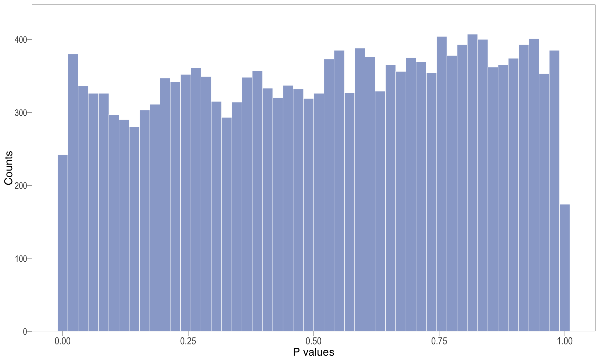

Version	Author	Date
d71eeb4	Ha Tran	2024-10-16

MA plot

| | | 0% | |………………………………………………………| 100% [ma_2]

.pl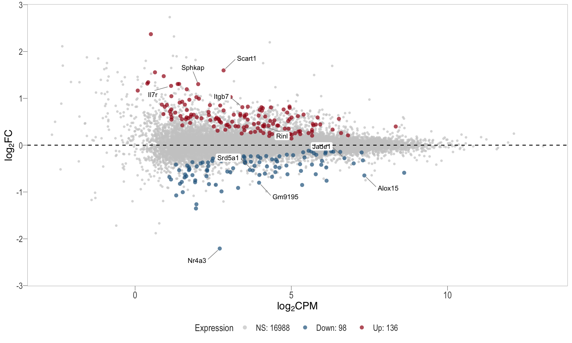

Version	Author	Date
d519e7f	Ha Tran	2024-12-03
d71eeb4	Ha Tran	2024-10-16

Volcano plot

| | | 0% | |……………………………………………………..| 100% [vol_2]

.pl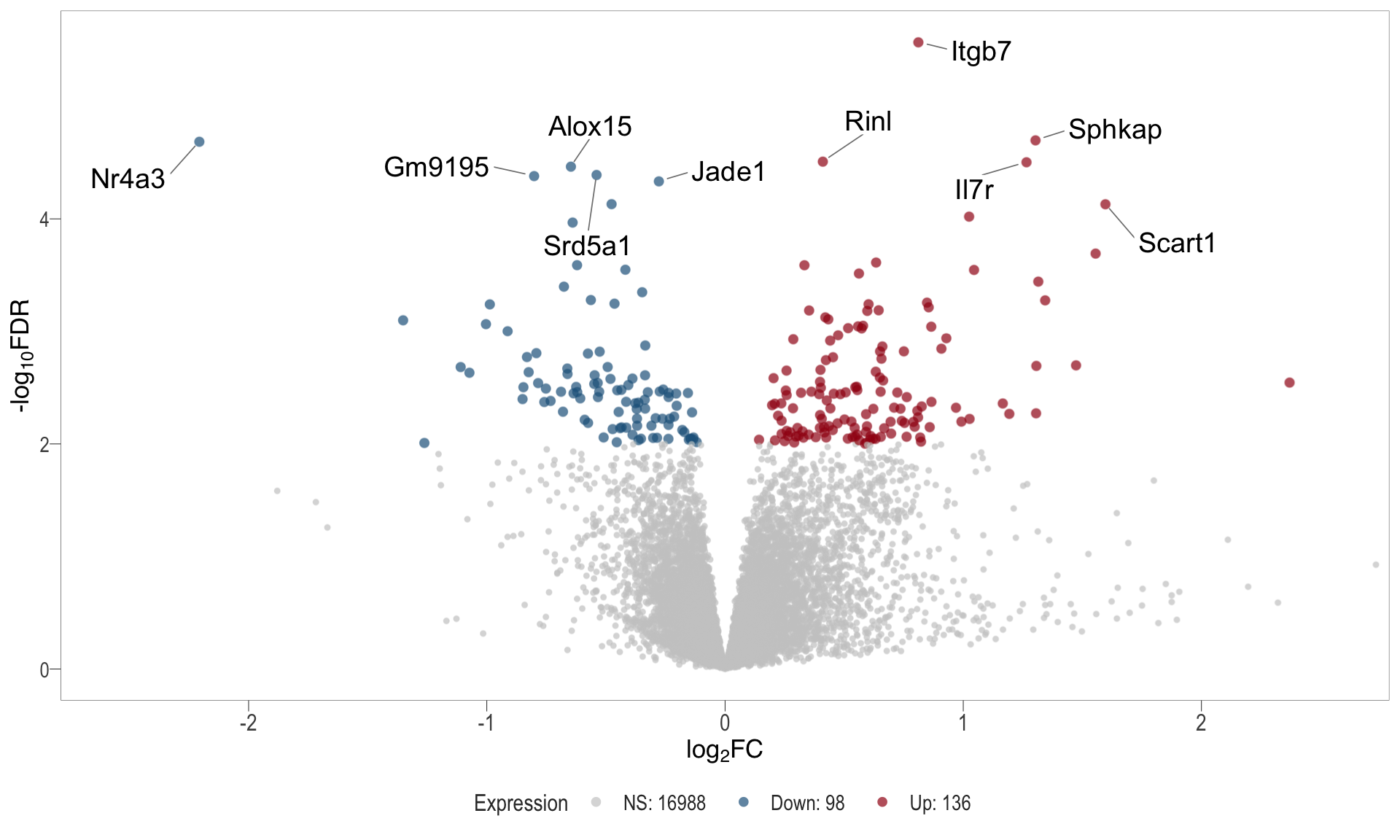

Version	Author	Date
d519e7f	Ha Tran	2024-12-03
d71eeb4	Ha Tran	2024-10-16

Top upregulated

| | | 0% | |…………………………………………………..| 100% [hmap_up2]

.pl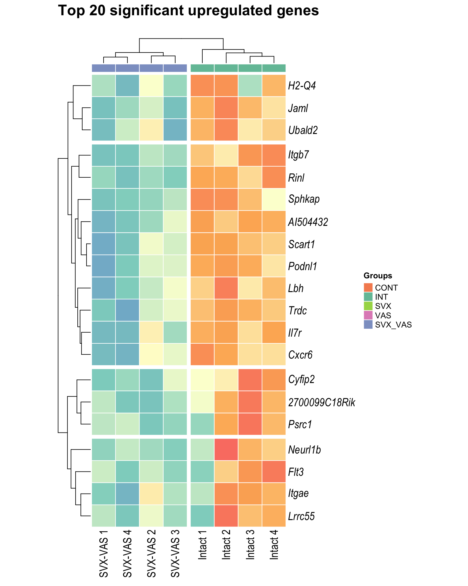

Version	Author	Date
d71eeb4	Ha Tran	2024-10-16

Top downregulated

| | | 0% | |…………………………………………………| 100% [hmap_down2]

.pl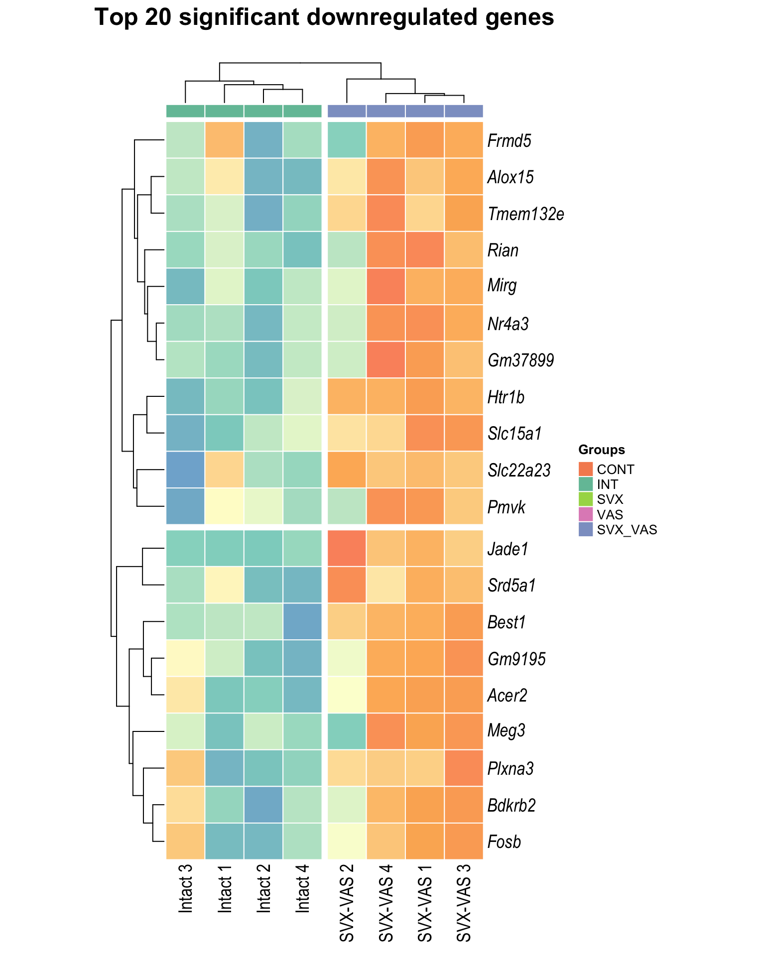

Version	Author	Date
d71eeb4	Ha Tran	2024-10-16

SVX vs SVX_VAS

P-val histogram

| | | 0% | |…………………………………………………….| 100% [hist_3]

.pl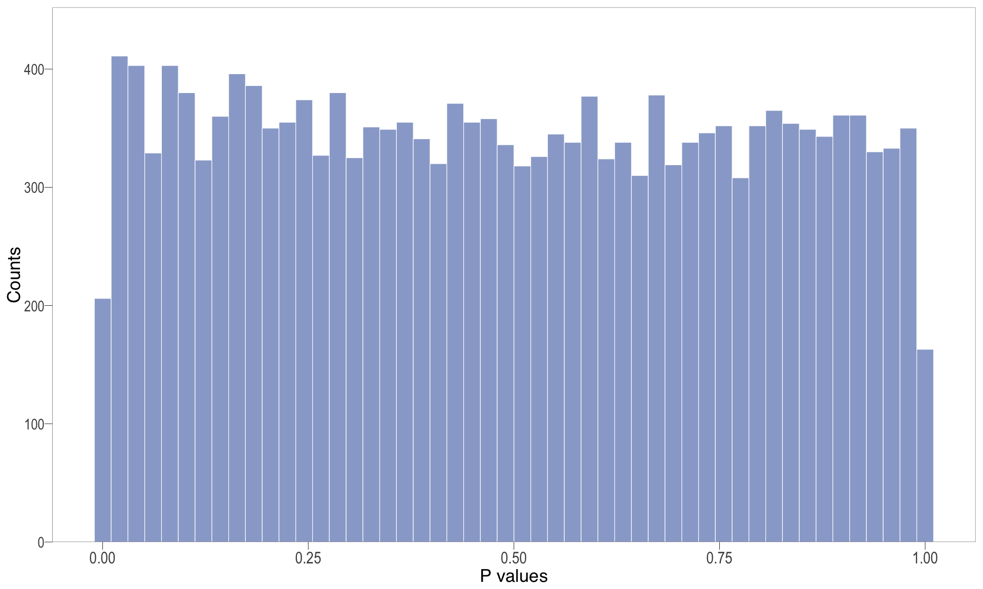

Version	Author	Date
d71eeb4	Ha Tran	2024-10-16

MA plot

| | | 0% | |………………………………………………………| 100% [ma_3]

.pl

Version	Author	Date
d519e7f	Ha Tran	2024-12-03
d71eeb4	Ha Tran	2024-10-16

Volcano plot

| | | 0% | |……………………………………………………..| 100% [vol_3]

.pl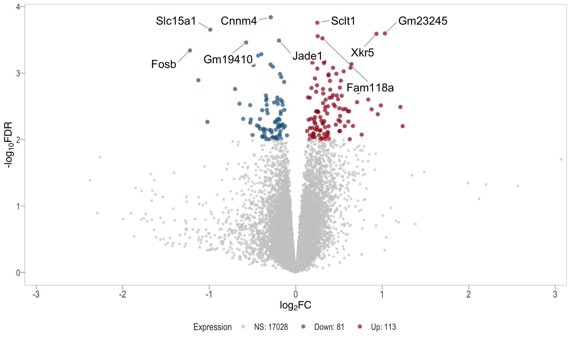

Version	Author	Date
d519e7f	Ha Tran	2024-12-03
d71eeb4	Ha Tran	2024-10-16

Top upregulated

| | | 0% | |…………………………………………………..| 100% [hmap_up3]

.pl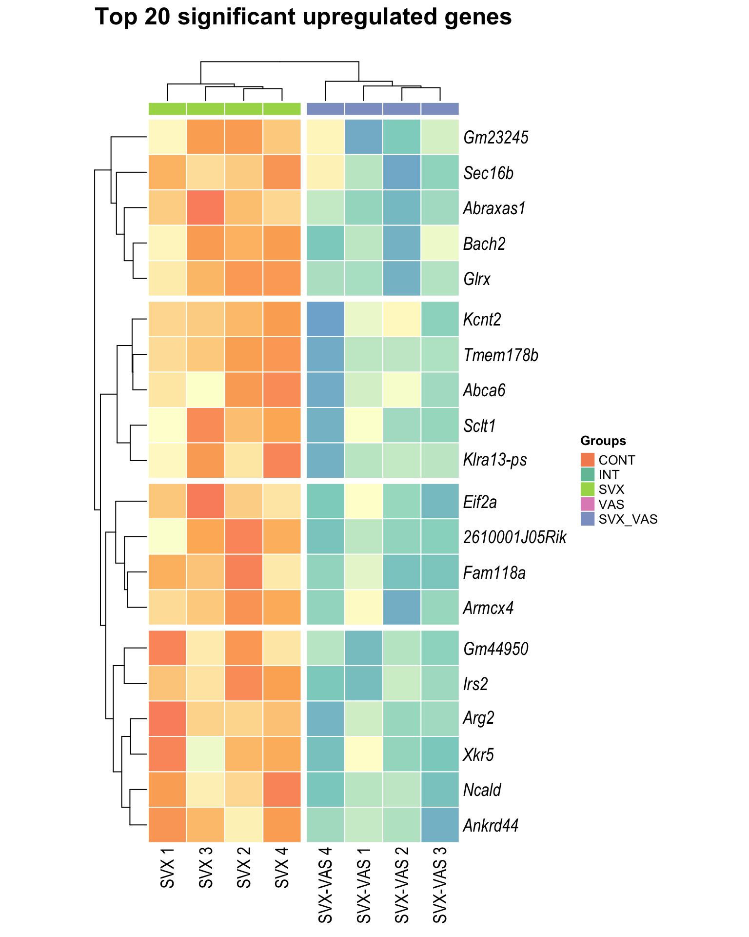

Version	Author	Date
d71eeb4	Ha Tran	2024-10-16

Top downregulated

| | | 0% | |…………………………………………………| 100% [hmap_down3]

.pl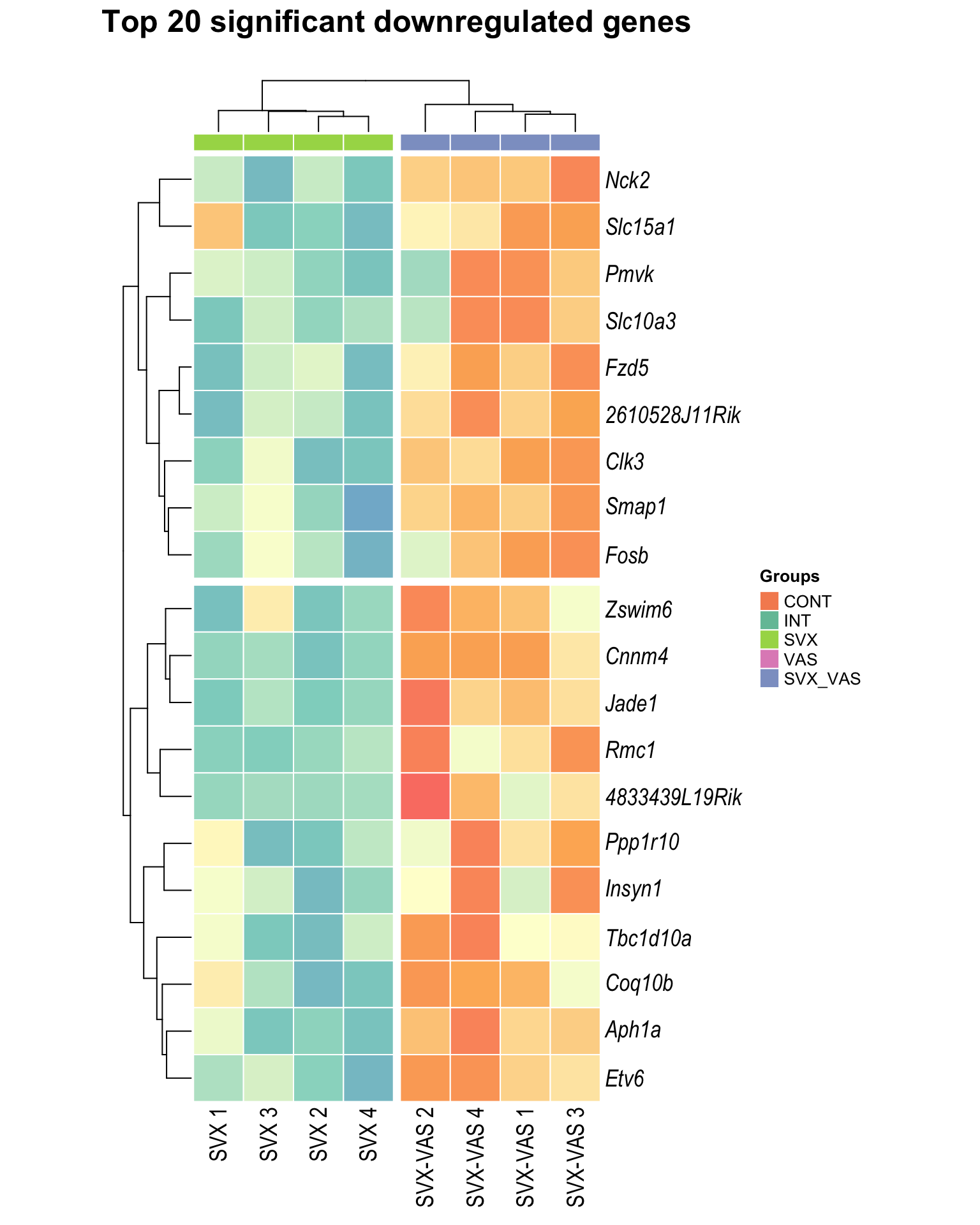

Version	Author	Date
d71eeb4	Ha Tran	2024-10-16

VAS vs SVX_VAS

P-val histogram

| | | 0% | |…………………………………………………….| 100% [hist_4]

.pl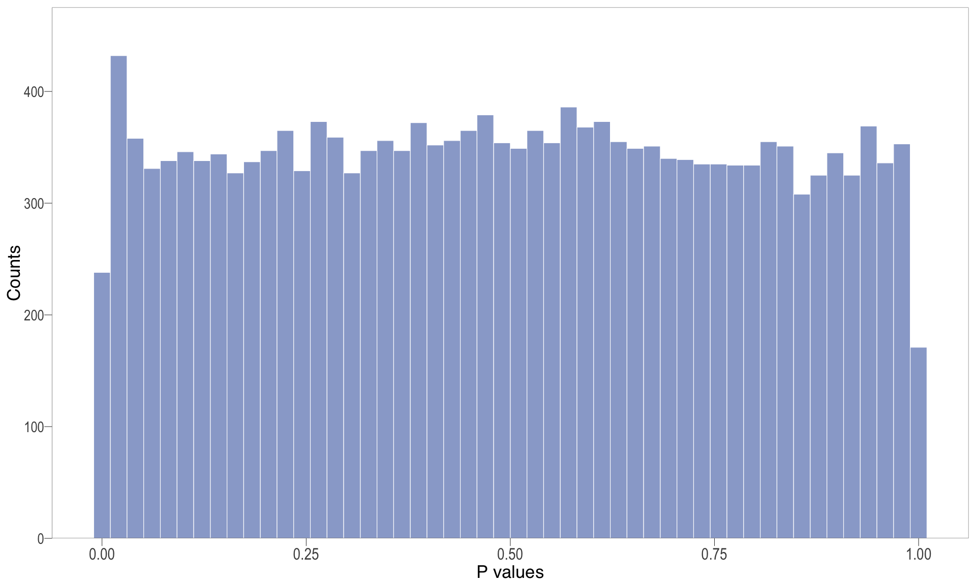

Version	Author	Date
d71eeb4	Ha Tran	2024-10-16

MA plot

| | | 0% | |………………………………………………………| 100% [ma_4]

.pl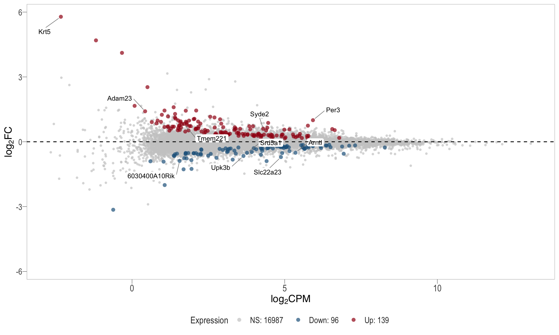

Version	Author	Date
d519e7f	Ha Tran	2024-12-03
d71eeb4	Ha Tran	2024-10-16

Volcano plot

| | | 0% | |……………………………………………………..| 100% [vol_4]

.pl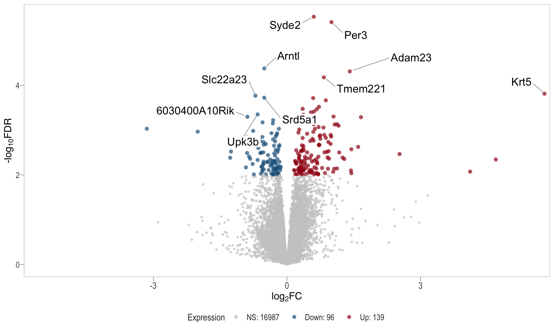

Version	Author	Date
d519e7f	Ha Tran	2024-12-03
d71eeb4	Ha Tran	2024-10-16

Top upregulated

| | | 0% | |…………………………………………………..| 100% [hmap_up4]

.pl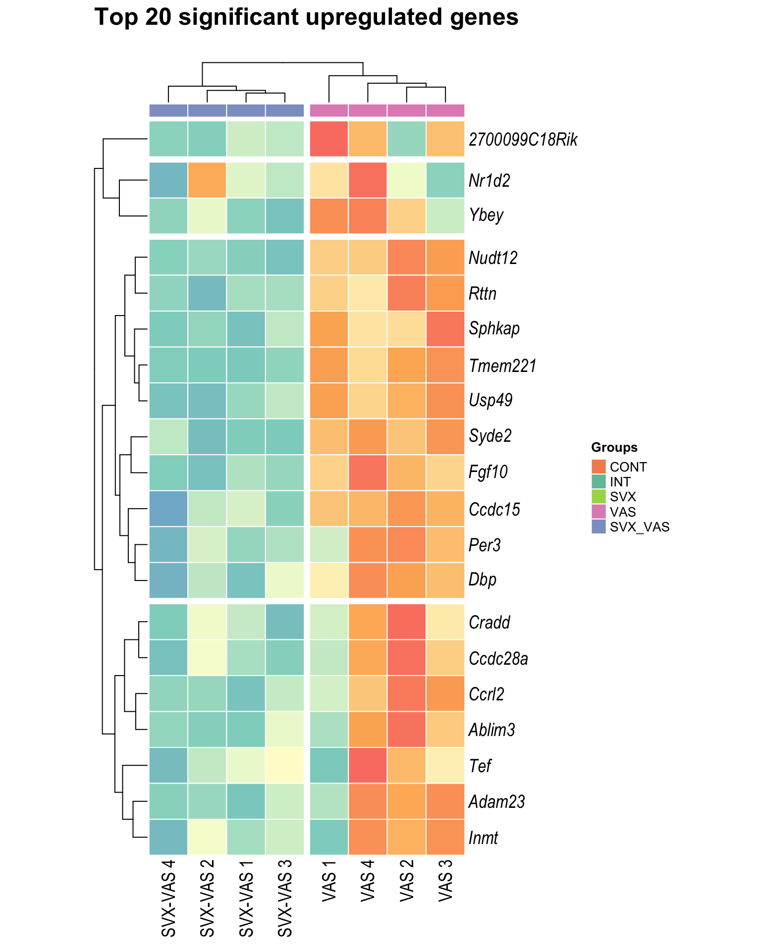

Version	Author	Date
d71eeb4	Ha Tran	2024-10-16

Top downregulated

| | | 0% | |…………………………………………………| 100% [hmap_down4]

.pl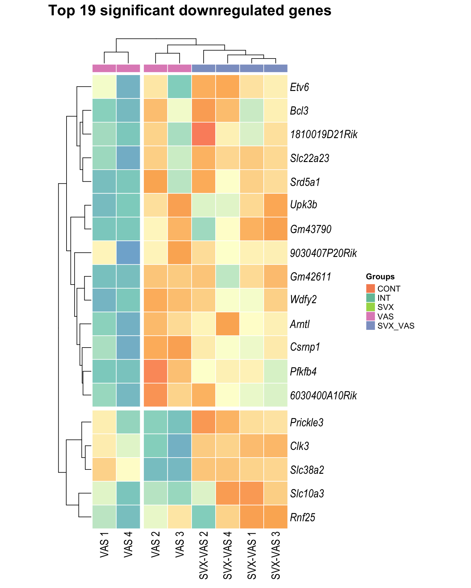

Version	Author	Date
d71eeb4	Ha Tran	2024-10-16

SVX_VAS vs CONT

P-val histogram

| | | 0% | |…………………………………………………….| 100% [hist_5]

.pl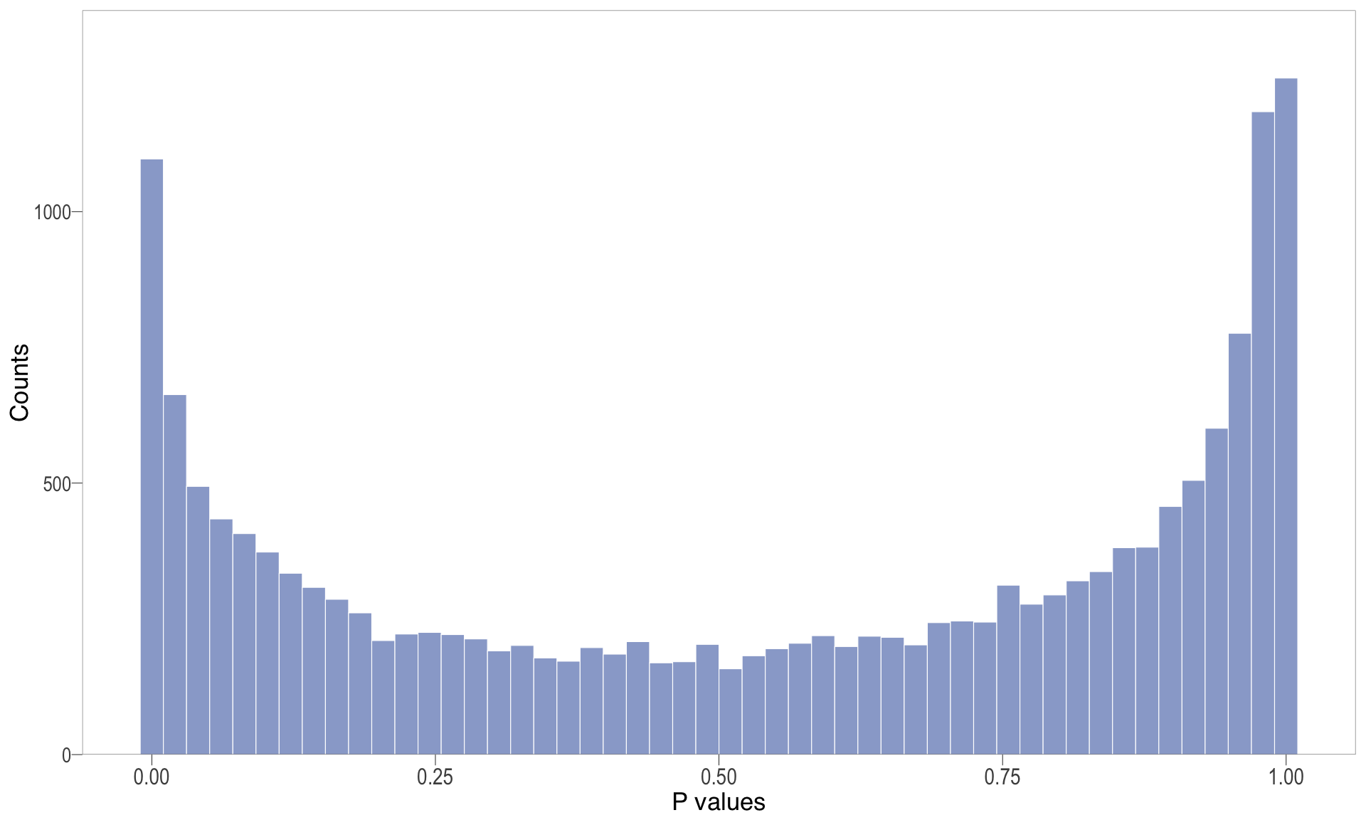

Version	Author	Date
d71eeb4	Ha Tran	2024-10-16

MA plot

| | | 0% | |………………………………………………………| 100% [ma_5]

.pl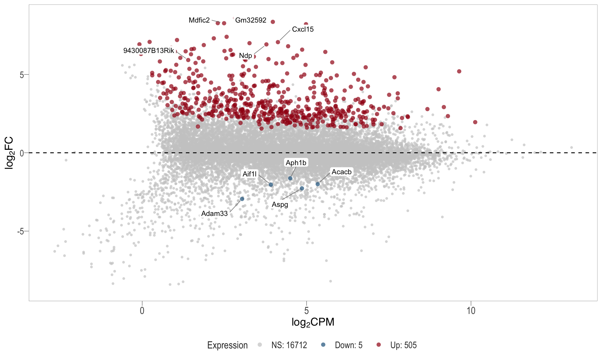

Version	Author	Date
d519e7f	Ha Tran	2024-12-03
d71eeb4	Ha Tran	2024-10-16

Volcano plot

| | | 0% | |……………………………………………………..| 100% [vol_5]

.pl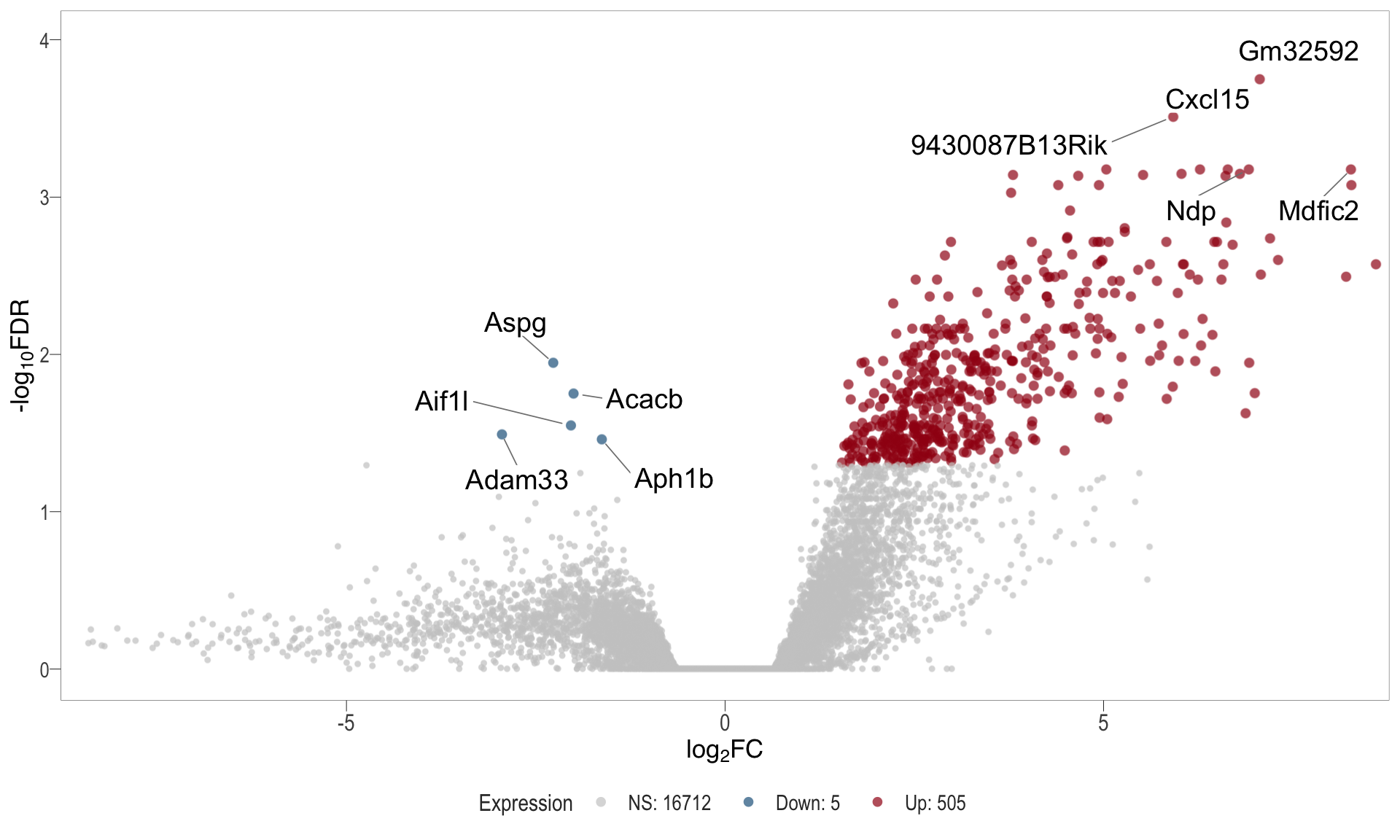

Version	Author	Date
d519e7f	Ha Tran	2024-12-03
d71eeb4	Ha Tran	2024-10-16

Top upregulated

| | | 0% | |…………………………………………………..| 100% [hmap_up5]

.pl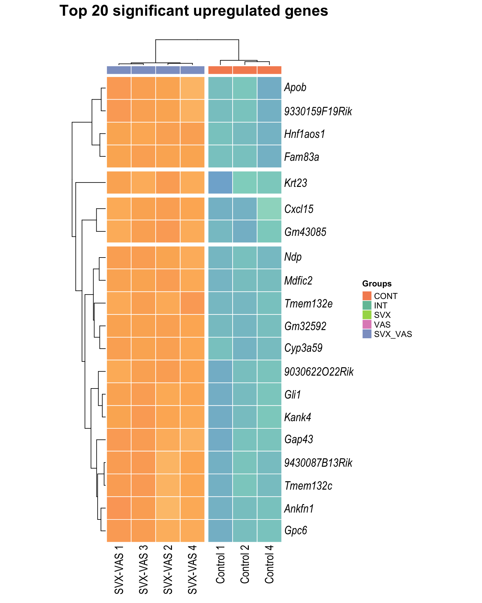

Version	Author	Date
d71eeb4	Ha Tran	2024-10-16

Top downregulated

| | | 0% | |…………………………………………………| 100% [hmap_down5]

.pl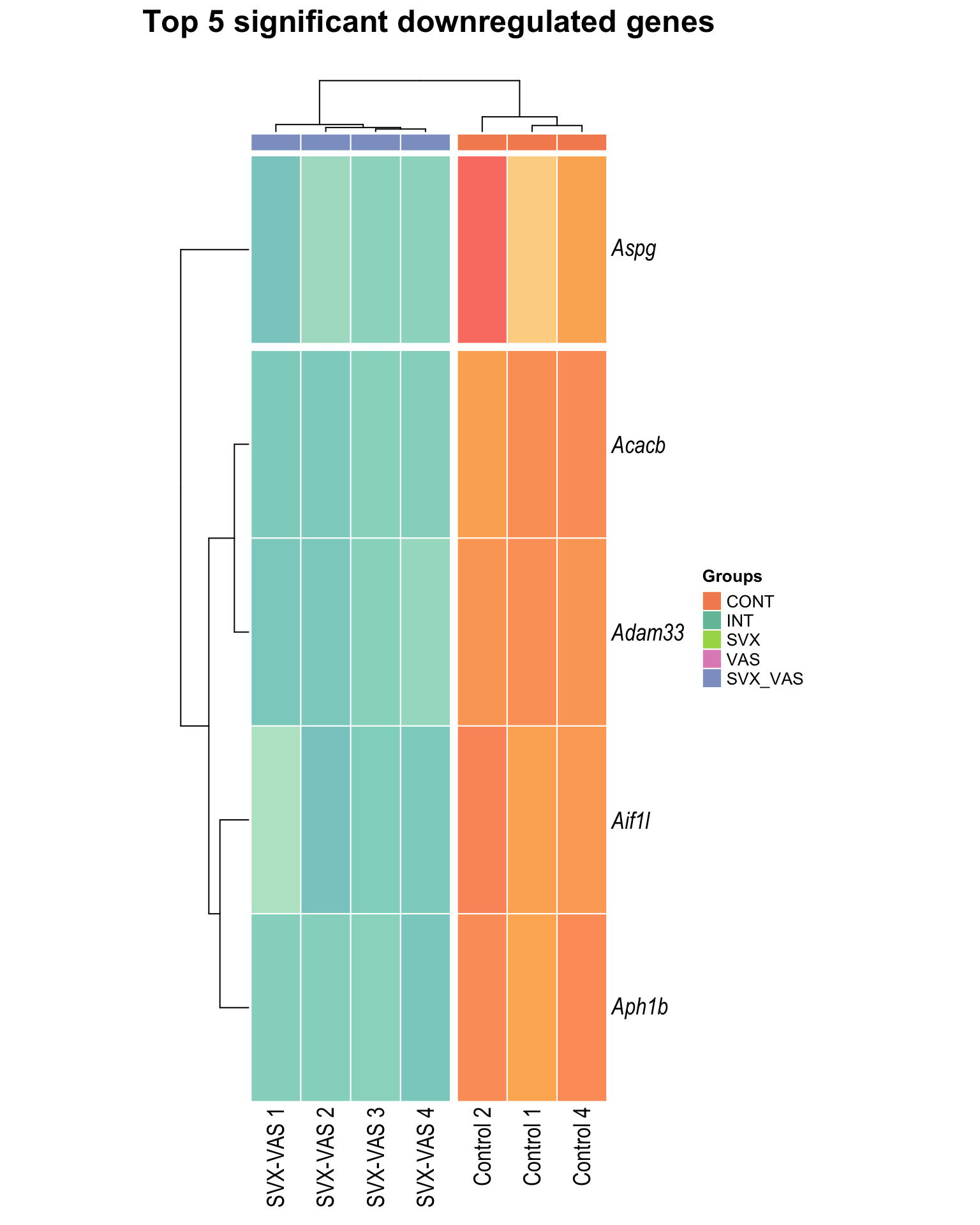

Version	Author	Date
d71eeb4	Ha Tran	2024-10-16

INT vs VAS

P-val histogram

| | | 0% | |…………………………………………………….| 100% [hist_6]

.pl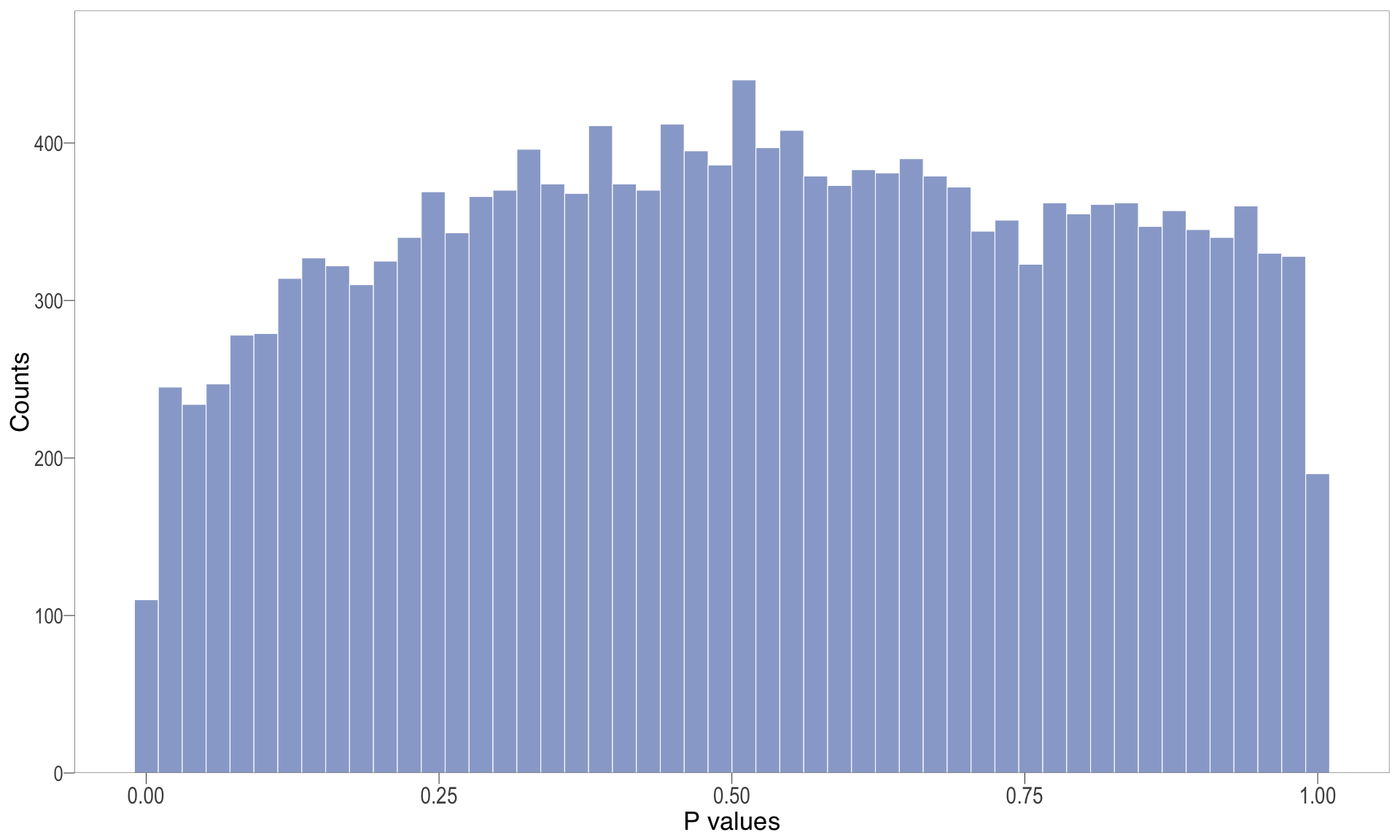

Version	Author	Date
d71eeb4	Ha Tran	2024-10-16

MA plot

| | | 0% | |………………………………………………………| 100% [ma_6]

.pl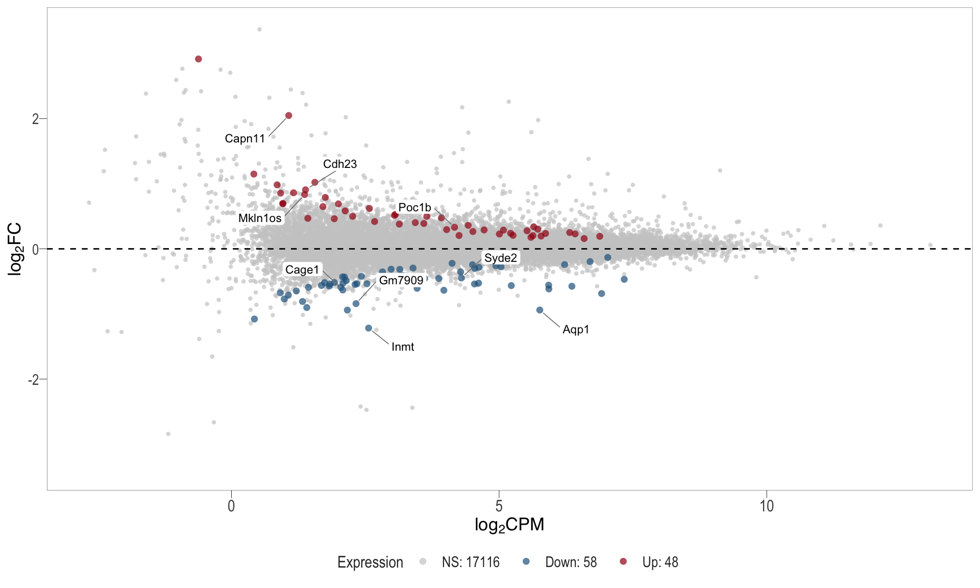

Version	Author	Date
d519e7f	Ha Tran	2024-12-03
d71eeb4	Ha Tran	2024-10-16

Volcano plot

| | | 0% | |……………………………………………………..| 100% [vol_6]

.pl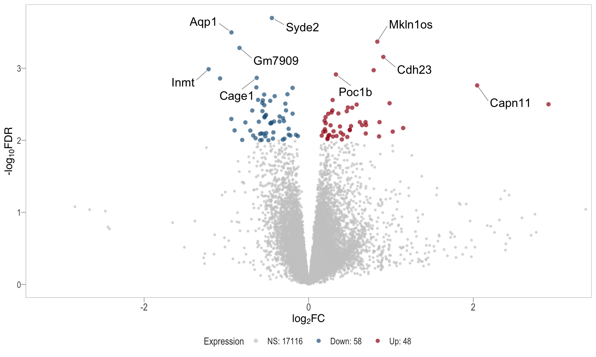

Version	Author	Date
d519e7f	Ha Tran	2024-12-03
d71eeb4	Ha Tran	2024-10-16

Top upregulated

| | | 0% | |…………………………………………………..| 100% [hmap_up6]

.pl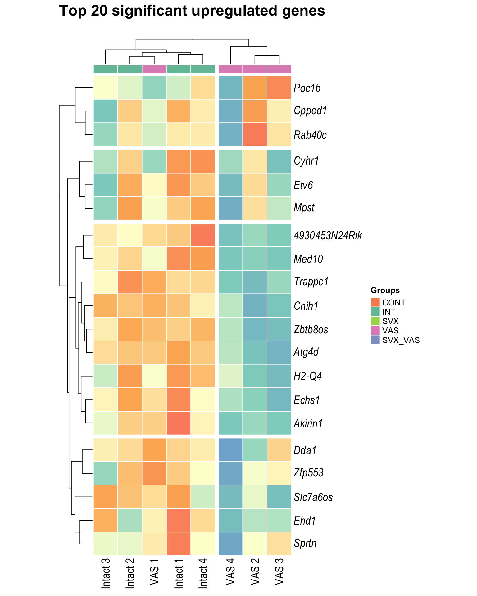

Version	Author	Date
d71eeb4	Ha Tran	2024-10-16

Top downregulated

| | | 0% | |…………………………………………………| 100% [hmap_down6]

.pl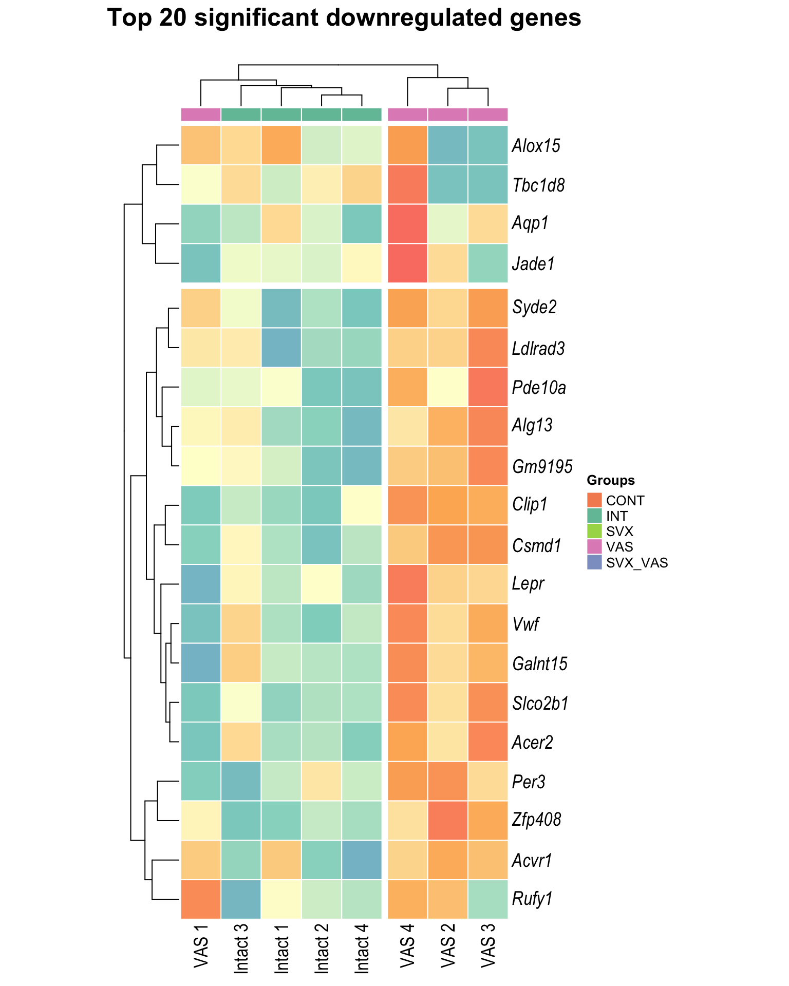

Version	Author	Date
d71eeb4	Ha Tran	2024-10-16

Combined

#create matrix with log cpm counts
logCPM <- cpm(dge, prior.count=2, log=TRUE)
rownames(logCPM) <- dge$genes$gene

#join common significant DE genes into df
common <- join_all(list(lm_sig[[1]], lm_sig[[2]], lm_sig[[3]],
                        lm_sig[[4]], lm_sig[[5]], lm_sig[[6]]), by = 'gene', type = 'inner')

Venn diagram

Heatmap

logCPM_combined <- cpm(dge, prior.count=3, log=TRUE)
rownames(logCPM_combined) <- dge$genes$gene_name

#join common significant DE genes into df
common <- join_all(list(lm_sig[[2]],lm_sig[[3]], lm_sig[[4]]), by = 'gene', type = 'inner')

#merge the log cpm counts with the top 30 common de genes
logCPM_combined <- logCPM_combined[common$gene_name[1:nrow(common)],]
logCPM_combined <- logCPM_combined[,c(4,5,6,7,16,17,18,19,8,9,10,11,12,13,14,15)]

#df for heatmap annotation of sample type
anno_combined <- factor(dge$samples$group, levels = c("INT", "VAS", "SVX", "SVX_VAS")) %>% as.data.frame()
anno_combined <- anno_combined[c(4,5,6,7,16,17,18,19,8,9,10,11,12,13,14,15),]%>% as.data.frame()

colnames(anno_combined) <- "Groups"

heat_combined <- ComplexHeatmap::pheatmap(
    mat = logCPM_combined,
    color = colorRampPalette(rev(c("#FB8072","#FDB462","#ffffd5","#8DD3C7","#80B1D3")))(300),
    scale = "row",
    cluster_cols = F,
    border_color = "white",
    gaps_col = c(4,8,12),
    cutree_cols = 5,
    cutree_rows = 6,
    treeheight_row = 40,
    treeheight_col = 30,
    show_colnames = T,
    clustering_distance_rows = "euclidean",
    # main = paste0("Top ", nrow(logCPM_combined), " significant DEGs"),

    legend = T,

    heatmap_legend_param = list(title = "Expression\nZ-score",
                                direction= "vertical",
                                merge_legend = T,
                                legend_direction = "vertical",
                                legend_width = unit(5, "cm")),

    # annotation = T,
    annotation_legend = T,
    annotation_col = anno_combined,
    annotation_colors = list("Groups" = groupColour),
    annotation_names_col = T,
    # annotation_legend_param = list(direction = "horizontal"),

    fontfamily = "Arial Narrow",
    fontsize = 12,
    fontsize_col = 12,
    fontsize_number = 12,
    fontsize_row = 12,
    labels_row = as.expression(lapply(rownames(logCPM_combined), function(a) bquote(italic(.(a)))))
  )


draw(heat_combined, merge_legend = T, heatmap_legend_side = "right", 
    annotation_legend_side = "right")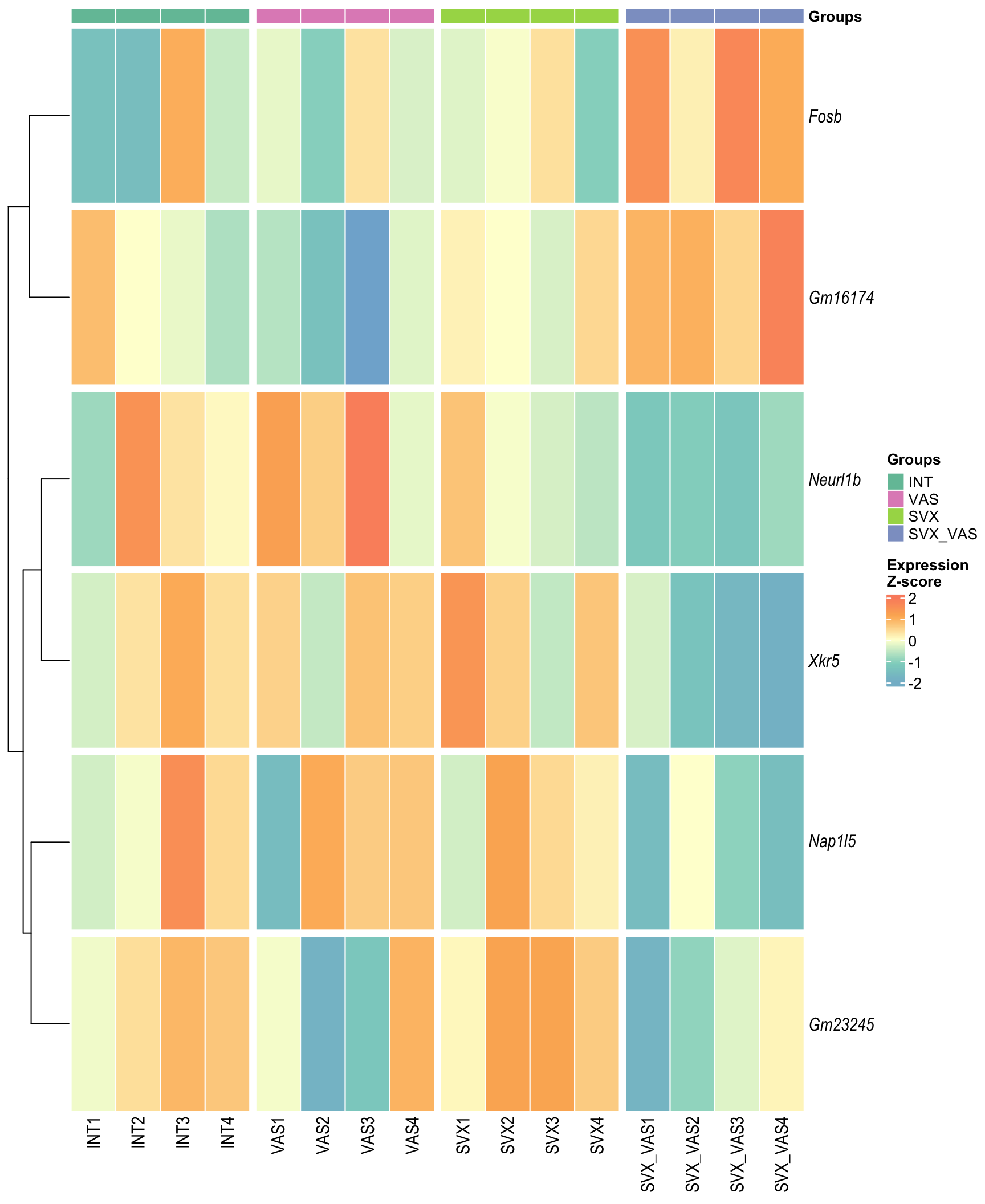

Version	Author	Date
d71eeb4	Ha Tran	2024-10-16

if (savePlots == T) {
  svg(filename = here::here("2_plots/2_DE/heat_combined.svg"),width = 8,height = 12)
  draw(heat_combined, merge_legend = T, heatmap_legend_side = "bottom", 
       annotation_legend_side = "bottom")
  dev.off()
  }

quartz_off_screen 
                2

Export Data

The following are exported:

de_genes_all.xlsx - This spreadsheet contains all DE genes.
de_genes_sig.xlsx - This spreadsheet contains only significant DE genes.

# export toptable for Dexter rewrite
# 
lapply(lm_all, function(x) x %>% dplyr::select(c("gene_name", "logFC", "AveExpr", "P.Value", "adj.P.Val", "description", "entrezid","expression"))) %>% writexl::write_xlsx(x = ., here::here("3_output/deg_all_new.xlsx"))

lapply(lm_sig, function(x) x %>% dplyr::select(c("gene_name", "logFC", "AveExpr", "P.Value", "adj.P.Val", "description", "entrezid","expression"))) %>% writexl::write_xlsx(x = ., here::here("3_output/deg_sig_new.xlsx"))

# save RDS object for enrichment analysis
saveRDS(object = comp, file = here::here("0_data/RDS_objects/comp.rds"))
saveRDS(object = lm, file = here::here("0_data/RDS_objects/lm.rds"))
saveRDS(object = lm_all, file = here::here("0_data/RDS_objects/lm_all.rds"))
saveRDS(object = lm_sig, file = here::here("0_data/RDS_objects/lm_sig.rds"))

writexl::write_xlsx(lapply(lm_sig[c(2,3,4)], function(x) { 
  degs <- x %>% remove_rownames() %>% dplyr::select(c("gene_name", "gene_biotype", "description", "logFC","AveExpr","t","P.Value","adj.P.Val", "gene", "entrezid")) 
  degs$description <- gsub("\\[.*?\\]", "", degs$description)
  return(degs)
}),path = here::here("3_output/DEGs.xlsx"))

t <- lapply(lm_sig[c(2,3,4)], function(x) { 
  degs <- x %>% remove_rownames() %>% dplyr::select(c("gene_name", "gene_biotype", "description", "logFC","AveExpr","t","P.Value","adj.P.Val", "gene", "entrezid")) 
  degs$description <- gsub("\\[.*?\\]", "", degs$description)
  return(degs)
  })

sessionInfo()

R version 4.4.1 (2024-06-14)
Platform: aarch64-apple-darwin20
Running under: macOS 26.1

Matrix products: default
BLAS:   /Library/Frameworks/R.framework/Versions/4.4-arm64/Resources/lib/libRblas.0.dylib 
LAPACK: /Library/Frameworks/R.framework/Versions/4.4-arm64/Resources/lib/libRlapack.dylib;  LAPACK version 3.12.0

locale:
[1] en_US.UTF-8/en_US.UTF-8/en_US.UTF-8/C/en_US.UTF-8/en_US.UTF-8

time zone: Australia/Adelaide
tzcode source: internal

attached base packages:
[1] grid      stats     graphics  grDevices utils     datasets  methods  
[8] base     

other attached packages:
 [1] knitr_1.50            ggrastr_1.0.2         pandoc_0.2.0         
 [4] Glimma_2.16.0         edgeR_4.4.2           limma_3.62.2         
 [7] viridis_0.6.5         viridisLite_0.4.2     ggrepel_0.9.6        
[10] ggpubr_0.6.1          ggplotify_0.1.3       extrafont_0.19       
[13] patchwork_1.3.2       DT_0.34.0             VennDiagram_1.7.3    
[16] futile.logger_1.4.3   pheatmap_1.0.13       cowplot_1.2.0        
[19] pander_0.6.6          kableExtra_1.4.0      plyr_1.8.9           
[22] scales_1.4.0          ComplexHeatmap_2.22.0 lubridate_1.9.4      
[25] forcats_1.0.0         stringr_1.5.2         purrr_1.1.0          
[28] tidyr_1.3.1           ggplot2_4.0.0         tidyverse_2.0.0      
[31] reshape2_1.4.4        tibble_3.3.0          readr_2.1.5          
[34] magrittr_2.0.4        dplyr_1.1.4           readxl_1.4.5         

loaded via a namespace (and not attached):
  [1] RColorBrewer_1.1-3          rstudioapi_0.17.1          
  [3] jsonlite_2.0.0              shape_1.4.6.1              
  [5] magick_2.9.0                ggbeeswarm_0.7.2           
  [7] farver_2.1.2                rmarkdown_2.29             
  [9] ragg_1.5.0                  zlibbioc_1.52.0            
 [11] GlobalOptions_0.1.2         fs_1.6.6                   
 [13] vctrs_0.6.5                 Cairo_1.6-5                
 [15] rstatix_0.7.2               S4Arrays_1.6.0             
 [17] htmltools_0.5.8.1           lambda.r_1.2.4             
 [19] broom_1.0.10                cellranger_1.1.0           
 [21] SparseArray_1.6.2           Formula_1.2-5              
 [23] gridGraphics_0.5-1          sass_0.4.10                
 [25] bslib_0.9.0                 htmlwidgets_1.6.4          
 [27] futile.options_1.0.1        cachem_1.1.0               
 [29] whisker_0.4.1               lifecycle_1.0.4            
 [31] iterators_1.0.14            pkgconfig_2.0.3            
 [33] Matrix_1.7-4                R6_2.6.1                   
 [35] fastmap_1.2.0               MatrixGenerics_1.18.1      
 [37] GenomeInfoDbData_1.2.13     clue_0.3-66                
 [39] digest_0.6.37               colorspace_2.1-1           
 [41] S4Vectors_0.44.0            DESeq2_1.46.0              
 [43] rprojroot_2.1.1             crosstalk_1.2.2            
 [45] textshaping_1.0.3           GenomicRanges_1.58.0       
 [47] labeling_0.4.3              timechange_0.3.0           
 [49] httr_1.4.7                  abind_1.4-8                
 [51] compiler_4.4.1              here_1.0.2                 
 [53] withr_3.0.2                 doParallel_1.0.17          
 [55] S7_0.2.0                    backports_1.5.0            
 [57] BiocParallel_1.40.2         carData_3.0-5              
 [59] Rttf2pt1_1.3.12             ggsignif_0.6.4             
 [61] DelayedArray_0.32.0         rappdirs_0.3.3             
 [63] rjson_0.2.23                tools_4.4.1                
 [65] vipor_0.4.7                 beeswarm_0.4.0             
 [67] httpuv_1.6.16               extrafontdb_1.0            
 [69] glue_1.8.0                  promises_1.3.3             
 [71] cluster_2.1.8.1             generics_0.1.4             
 [73] gtable_0.3.6                tzdb_0.5.0                 
 [75] hms_1.1.3                   XVector_0.46.0             
 [77] xml2_1.4.0                  car_3.1-3                  
 [79] BiocGenerics_0.52.0         foreach_1.5.2              
 [81] pillar_1.11.1               yulab.utils_0.2.1          
 [83] later_1.4.4                 circlize_0.4.16            
 [85] lattice_0.22-7              tidyselect_1.2.1           
 [87] locfit_1.5-9.12             git2r_0.36.2               
 [89] gridExtra_2.3               IRanges_2.40.1             
 [91] SummarizedExperiment_1.36.0 svglite_2.2.1              
 [93] stats4_4.4.1                xfun_0.53                  
 [95] Biobase_2.66.0              statmod_1.5.0              
 [97] matrixStats_1.5.0           stringi_1.8.7              
 [99] UCSC.utils_1.2.0            workflowr_1.7.2            
[101] yaml_2.3.10                 evaluate_1.0.5             
[103] codetools_0.2-20            cli_3.6.5                  
[105] systemfonts_1.2.3           jquerylib_0.1.4            
[107] Rcpp_1.1.0                  GenomeInfoDb_1.42.3        
[109] png_0.1-8                   parallel_4.4.1             
[111] writexl_1.5.4               crayon_1.5.3               
[113] GetoptLong_1.0.5            rlang_1.1.6                
[115] formatR_1.14

DE Analysis

Ha Tran

22/08/2021

Data Setup

Import DGElist Data

Initial Parameterisation

Design Matrix

Contrast Matrix

Limma-Voom

Apply voom transformation

Observational-level weights

Observational and group level weights

Observational and sample level weights

Visualisation of Voom transformation

Groups and sample weights

PCA

Apply linear model

FC=none

FC=1.1

FC=1.2

FC=1.5

Differential Gene Expression analysis

INT vs CONT

P-val histogram

MA plot

Volcano plot

Top upregulated

Top downregulated

INT vs SVX_VAS

P-val histogram

MA plot

Volcano plot

Top upregulated

Top downregulated

SVX vs SVX_VAS

P-val histogram

MA plot

Volcano plot

Top upregulated

Top downregulated

VAS vs SVX_VAS

P-val histogram

MA plot

Volcano plot

Top upregulated

Top downregulated

SVX_VAS vs CONT

P-val histogram

MA plot

Volcano plot

Top upregulated

Top downregulated

INT vs VAS

P-val histogram

MA plot

Volcano plot

Top upregulated

Top downregulated

Combined

Venn diagram

Heatmap

Export Data