Additional Figures
Ha Tran
24/12/2021
Last updated: 2025-11-27
Checks: 7 0
Knit directory: 5_gd_Tcell/1_analysis/
This reproducible R Markdown analysis was created with workflowr (version 1.7.2). The Checks tab describes the reproducibility checks that were applied when the results were created. The Past versions tab lists the development history.
Great! Since the R Markdown file has been committed to the Git repository, you know the exact version of the code that produced these results.
Great job! The global environment was empty. Objects defined in the global environment can affect the analysis in your R Markdown file in unknown ways. For reproduciblity it’s best to always run the code in an empty environment.
The command set.seed(12345) was run prior to running the
code in the R Markdown file. Setting a seed ensures that any results
that rely on randomness, e.g. subsampling or permutations, are
reproducible.
Great job! Recording the operating system, R version, and package versions is critical for reproducibility.
Nice! There were no cached chunks for this analysis, so you can be confident that you successfully produced the results during this run.
Great job! Using relative paths to the files within your workflowr project makes it easier to run your code on other machines.
Great! You are using Git for version control. Tracking code development and connecting the code version to the results is critical for reproducibility.
The results in this page were generated with repository version b9f184a. See the Past versions tab to see a history of the changes made to the R Markdown and HTML files.
Note that you need to be careful to ensure that all relevant files for
the analysis have been committed to Git prior to generating the results
(you can use wflow_publish or
wflow_git_commit). workflowr only checks the R Markdown
file, but you know if there are other scripts or data files that it
depends on. Below is the status of the Git repository when the results
were generated:
Ignored files:
    Ignored:    .Rhistory
    Ignored:    .Rproj.user/

Untracked files:
    Untracked:  .DS_Store
    Untracked:  figure/scatter2-1.png
    Untracked:  figure/scatter3-1.png
    Untracked:  figure/scatter4-1.png
    Untracked:  figure/scatter5-1.png
    Untracked:  figure/scatter_3d4-1.png
    Untracked:  figure/scatter_interactive4-1.png
    Untracked:  figure/treemap2-1.png
    Untracked:  figure/treemap3-1.png
    Untracked:  figure/treemap4-1.png
    Untracked:  figure/treemap5-1.png

Unstaged changes:
    Modified:   0_data/RDS_plots/go_combined_dotPlot.rds
    Modified:   0_data/RDS_plots/go_combined_parTerm_dotPlot.rds
    Modified:   0_data/RDS_plots/go_dotPlot.rds
    Modified:   0_data/RDS_plots/go_parTerm_dotPlot.rds
    Modified:   0_data/RDS_plots/go_parTerm_scatter.rds
    Modified:   0_data/RDS_plots/kegg_dotPlot.rds
    Modified:   0_data/RDS_plots/kegg_path_Hmap.rds
    Modified:   0_data/RDS_plots/ma_plots.rds
    Modified:   0_data/RDS_plots/react_combined_dotPlot.rds
    Modified:   0_data/RDS_plots/react_dotPlot.rds
    Modified:   0_data/RDS_plots/vol_plots.rds
    Modified:   2_plots/1_QC/PC1_PC2.svg
    Modified:   2_plots/1_QC/PC1_PC3.svg
    Modified:   2_plots/1_QC/PC2_PC3.svg
    Modified:   2_plots/2_DE/heat_down_INT vs CONT.svg
    Modified:   2_plots/2_DE/heat_down_INT vs SVX_VAS.svg
    Modified:   2_plots/2_DE/heat_down_INT vs VAS.svg
    Modified:   2_plots/2_DE/heat_down_SVX vs SVX_VAS.svg
    Modified:   2_plots/2_DE/heat_down_SVX_VAS vs CONT.svg
    Modified:   2_plots/2_DE/heat_down_VAS vs SVX_VAS.svg
    Modified:   2_plots/2_DE/heat_up_INT vs CONT.svg
    Modified:   2_plots/2_DE/heat_up_INT vs SVX_VAS.svg
    Modified:   2_plots/2_DE/heat_up_INT vs VAS.svg
    Modified:   2_plots/2_DE/heat_up_SVX vs SVX_VAS.svg
    Modified:   2_plots/2_DE/heat_up_SVX_VAS vs CONT.svg
    Modified:   2_plots/2_DE/heat_up_VAS vs SVX_VAS.svg
    Modified:   2_plots/2_DE/hist_INT vs CONT.svg
    Modified:   2_plots/2_DE/hist_INT vs SVX_VAS.svg
    Modified:   2_plots/2_DE/hist_INT vs VAS.svg
    Modified:   2_plots/2_DE/hist_SVX vs SVX_VAS.svg
    Modified:   2_plots/2_DE/hist_SVX_VAS vs CONT.svg
    Modified:   2_plots/2_DE/hist_VAS vs SVX_VAS.svg
    Modified:   2_plots/3_FA/go/combine_go_dot.svg
    Modified:   2_plots/3_FA/go/parTerm_dot_INT vs CONT.svg
    Modified:   2_plots/3_FA/go/parTerm_dot_INT vs SVX_VAS.svg
    Modified:   2_plots/3_FA/go/parTerm_dot_SVX vs SVX_VAS.svg
    Modified:   2_plots/3_FA/go/parTerm_dot_SVX_VAS vs CONT.svg
    Modified:   2_plots/3_FA/go/parTerm_dot_VAS vs SVX_VAS.svg
    Modified:   2_plots/3_FA/go/semSim_dendrogram_INT vs CONT.svg
    Modified:   2_plots/3_FA/go/semSim_dendrogram_INT vs SVX_VAS.svg
    Modified:   2_plots/3_FA/go/semSim_dendrogram_SVX vs SVX_VAS.svg
    Modified:   2_plots/3_FA/go/semSim_dendrogram_SVX_VAS vs CONT.svg
    Modified:   2_plots/3_FA/go/semSim_dendrogram_VAS vs SVX_VAS.svg
    Modified:   2_plots/3_FA/go/semSim_scatter_INT vs CONT.svg
    Modified:   2_plots/3_FA/go/semSim_scatter_INT vs SVX_VAS.svg
    Modified:   2_plots/3_FA/go/semSim_scatter_SVX vs SVX_VAS.svg
    Modified:   2_plots/3_FA/go/semSim_scatter_SVX_VAS vs CONT.svg
    Modified:   2_plots/3_FA/kegg/combine_kegg_dot.svg
    Modified:   2_plots/3_FA/kegg/heat_Neutrophil extracellular trap formation.svg
    Modified:   2_plots/3_FA/kegg/heat_PD-L1 expression and PD-1 checkpoint pathway in cancer.svg
    Modified:   2_plots/3_FA/kegg/heat_T cell receptor signaling pathway.svg
    Modified:   2_plots/3_FA/kegg/heat_Th1 and Th2 cell differentiation.svg
    Modified:   2_plots/3_FA/kegg/heat_Th17 cell differentiation.svg
    Modified:   2_plots/3_FA/kegg/kegg_dot_INT vs CONT.svg
    Modified:   2_plots/3_FA/kegg/kegg_dot_INT vs SVX_VAS.svg
    Modified:   2_plots/3_FA/kegg/kegg_dot_SVX_VAS vs CONT.svg
    Modified:   2_plots/3_FA/kegg/kegg_dot_VAS vs SVX_VAS.svg
    Modified:   2_plots/3_FA/kegg/kegg_upset_INT vs CONT.svg
    Modified:   2_plots/3_FA/kegg/kegg_upset_INT vs SVX_VAS.svg
    Modified:   2_plots/3_FA/kegg/kegg_upset_SVX_VAS vs CONT.svg
    Modified:   2_plots/3_FA/kegg/kegg_upset_VAS vs SVX_VAS.svg
    Modified:   2_plots/3_FA/reactome/combine_react_dot.svg
    Modified:   2_plots/3_FA/reactome/react_dot_INT vs CONT.svg
    Modified:   2_plots/3_FA/reactome/react_dot_INT vs SVX_VAS.svg
    Modified:   2_plots/3_FA/reactome/react_dot_INT vs VAS.svg
    Modified:   2_plots/3_FA/reactome/react_dot_SVX vs SVX_VAS.svg
    Modified:   2_plots/3_FA/reactome/react_dot_SVX_VAS vs CONT.svg
    Modified:   2_plots/3_FA/reactome/react_dot_VAS vs SVX_VAS.svg
    Modified:   2_plots/3_FA/reactome/react_upset_INT vs CONT.svg
    Modified:   2_plots/3_FA/reactome/react_upset_INT vs SVX_VAS.svg
    Modified:   2_plots/3_FA/reactome/react_upset_INT vs VAS.svg
    Modified:   2_plots/3_FA/reactome/react_upset_SVX vs SVX_VAS.svg
    Modified:   2_plots/3_FA/reactome/react_upset_SVX_VAS vs CONT.svg
    Modified:   2_plots/3_FA/reactome/react_upset_VAS vs SVX_VAS.svg
    Modified:   2_plots/4_paper/subset_degs.svg
    Modified:   2_plots/combine_ipa_dot.svg
    Modified:   2_plots/dnf_plot.svg
    Modified:   2_plots/intVsvxVAS.svg
    Modified:   2_plots/upstream_hmap.svg
    Modified:   3_output/DEGs.xlsx
    Modified:   3_output/Gene Ontology.xlsx
    Modified:   3_output/KEGG.xlsx
    Modified:   3_output/Reactome.xlsx
    Modified:   3_output/deg_all_new.xlsx
    Modified:   3_output/deg_sig_new.xlsx
    Modified:   3_output/eigenvalues.xlsx
    Modified:   3_output/enrichKEGG_sig.xlsx
    Modified:   3_output/reactome_all_new.xlsx
    Modified:   3_output/reactome_sig_new.xlsx
    Modified:   3_output/semSim_GO_sig.xlsx
    Modified:   README.html
    Modified:   README.md
    Modified:   figure/dot2-1.png
    Modified:   figure/dot3-1.png
    Modified:   figure/dot4-1.png
    Modified:   figure/dot5-1.png
    Modified:   figure/upset2-1.png
    Modified:   figure/upset3-1.png
    Modified:   figure/upset4-1.png
    Modified:   figure/upset5-1.png
Note that any generated files, e.g. HTML, png, CSS, etc., are not included in this status report because it is ok for generated content to have uncommitted changes.
These are the previous versions of the repository in which changes were
made to the R Markdown (1_analysis/extraFigures.Rmd) and
HTML (docs/extraFigures.html) files. If you’ve configured a
remote Git repository (see ?wflow_git_remote), click on the
hyperlinks in the table below to view the files as they were in that
past version.
| File | Version | Author | Date | Message |
|---|---|---|---|---|
| html | d519e7f | Ha Tran | 2024-12-03 | Build site. |
| Rmd | 9fc0156 | Ha Tran | 2024-12-03 | workflowr::wflow_publish(here::here("1_analysis/*.Rmd")) |
| html | 5dce909 | Ha Tran | 2024-11-07 | Build site. |
| Rmd | 6b2e610 | Ha Tran | 2024-11-07 | workflowr::wflow_publish(here::here("1_analysis/*.Rmd")) |
| html | d71eeb4 | Ha Tran | 2024-10-16 | Build site. |
| html | ae93fcc | tranmanhha135 | 2024-02-02 | Build site. |
| Rmd | fbcdd69 | tranmanhha135 | 2024-02-02 | workflowr::wflow_publish(here::here("1_analysis/*.Rmd")) |
| Rmd | ccb39d7 | tranmanhha135 | 2022-10-22 | safety commit |
| Rmd | 2c24612 | tranmanhha135 | 2022-10-13 | build website |
| html | 2c24612 | tranmanhha135 | 2022-10-13 | build website |
| Rmd | 866017e | tranmanhha135 | 2022-10-13 | minor changes |
| Rmd | 324032b | tranmanhha135 | 2022-10-11 | resize images |
| Rmd | 43675d3 | tranmanhha135 | 2022-10-06 | Add IPA data |
| html | 43675d3 | tranmanhha135 | 2022-10-06 | Add IPA data |
| html | 11a5cf4 | tranmanhha135 | 2022-10-03 | build wedsite |
| Rmd | 192d010 | tranmanhha135 | 2022-09-20 | functional enrichment with new dataset |
| Rmd | 0df047f | tranmanhha135 | 2022-09-08 | minor changes to build and publish |
| html | 0df047f | tranmanhha135 | 2022-09-08 | minor changes to build and publish |
| Rmd | 889dfb5 | Ha Tran | 2022-01-01 | changed colour scheme, minor cosmetic changes |
| html | 889dfb5 | Ha Tran | 2022-01-01 | changed colour scheme, minor cosmetic changes |
| html | 54e0166 | Ha Manh Tran | 2022-01-01 | Build site. |
| html | 32454d5 | Ha Manh Tran | 2022-01-01 | Build site. |
| Rmd | c667dd0 | Ha Manh Tran | 2022-01-01 | workflowr::wflow_publish(files = here::here(c("1_analysis/index.Rmd", |
# load DGElist previously created in the set up
# dge <- readRDS(here::here("0_data/RDS_objects/dge.rds"))
lm <- readRDS(here::here("0_data/RDS_objects/lm.rds"))
lm_all <- readRDS(here::here("0_data/RDS_objects/lm_all.rds"))
lm_sig <- readRDS(here::here("0_data/RDS_objects/lm_sig.rds"))
# Comp <- readRDS(here::here("0_data/RDS_objects/comp.rds"))
# to increase the knitting speed. change to T to save all plots
savePlots <- T
export <- T
# Theme
bossTheme <- readRDS(here::here("0_data/functions/bossTheme.rds"))
bossTheme_bar <- readRDS(here::here("0_data/functions/bossTheme_bar.rds"))
groupColour <- readRDS(here::here("0_data/functions/groupColour.rds"))
groupColour_dark <- readRDS(here::here("0_data/functions/groupColour_dark.rds"))
expressionCol <- readRDS(here::here("0_data/functions/expressionCol.rds"))
expressionCol_dark <- readRDS(here::here("0_data/functions/expressionCol_dark.rds"))
compColour <- readRDS(here::here("0_data/functions/compColour.rds"))
DT <- readRDS(here::here("0_data/functions/DT.rds"))
# Plotting
convert_to_superscript <- readRDS(here::here("0_data/functions/convert_to_superscript.rds"))
exponent <- readRDS(here::here("0_data/functions/exponent.rds"))
format_y_axis <- readRDS(here::here("0_data/functions/format_y_axis.rds"))
firstCap <- function(x) {
substr(x, 1, 1) <- toupper(substr(x, 1, 1))
x
}IPA analysis
Regulated Pathways
read_excel_allsheets <- function(filename, tibble = FALSE) {
sheets <- readxl::excel_sheets(filename)
x <- lapply(sheets, function(X) readxl::read_excel(filename, sheet = X))
if(!tibble) x <- lapply(x, as.data.frame)
names(x) <- sheets
x
}
pathways <- read_excel_allsheets(here::here("0_data/raw_data/IPA_pathways.xlsx"))
pathways <- lapply(pathways, function(x) {
colnames(x) <- c("name", "logPval", "pval", "ratio", "zScore", "molecules")
x <- x %>% dplyr::mutate(pval = 10^-logPval, .after = logPval)
x$name <- x$name %>% firstCap() %>% str_wrap(width = 45)
return(x)
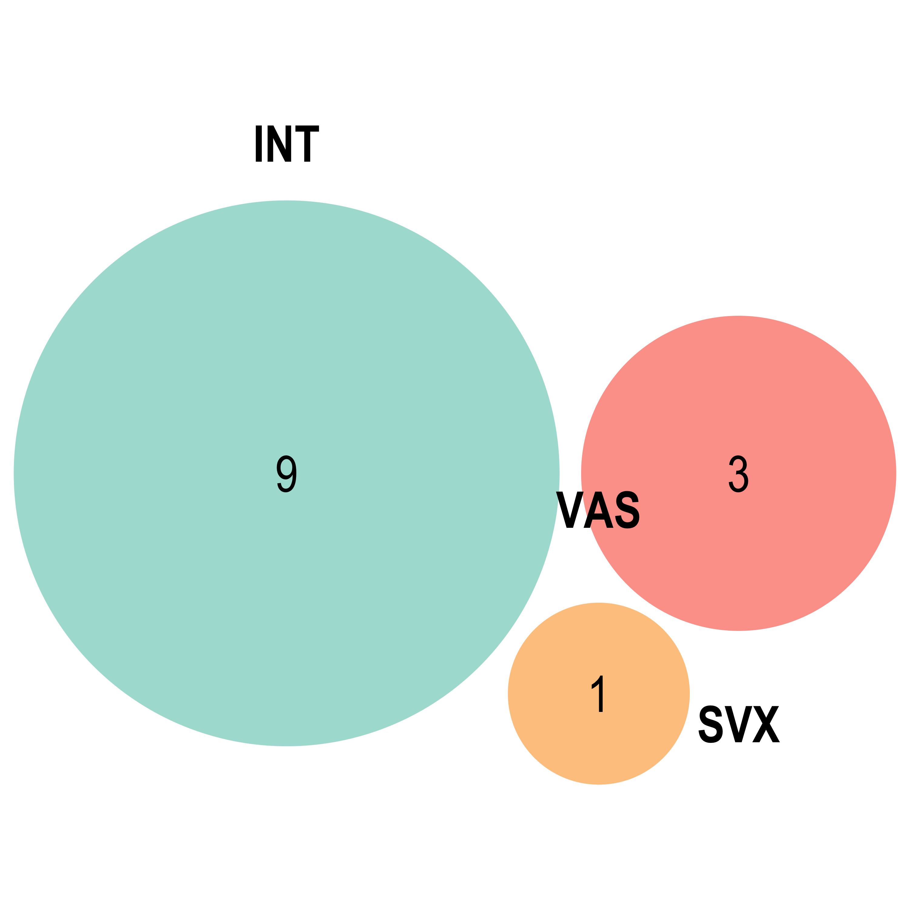
})Venn diagram
Dot plot
# combine all df in list into one df
library(stringi)
ipa_dot_all <- as.data.frame(do.call(rbind, pathways)) %>%
  rownames_to_column("group")

ipa_dot_all$group <- gsub(pattern = "\\..*", "", ipa_dot_all$group) %>% as.factor()

# remove the " vs SVX_VAS" from group name
ipa_dot_all$group <- gsub(pattern = " vs SVX_VAS", "", ipa_dot_all$group) %>% as.factor()


# clean group names and change to factor
ipa_dot_all$group <- factor(ipa_dot_all$group,levels = c("INT", "SVX", "VAS"))
ipa_dot_all <- ipa_dot_all %>% dplyr::mutate(count = stri_count(molecules,fixed = ",") + 1,
                                             state = case_when(zScore < 0 ~ "Decreased",
                                                               zScore > 0 ~ "Increased",
                                                               TRUE ~ "NA"))
ipa_dot_all$name <- ipa_dot_all$name %>% str_wrap(28)

ipa_dot_all$name <- factor(ipa_dot_all$name, levels = unique(ipa_dot_all$name[order(ipa_dot_all$zScore, decreasing = F)]))

path_dot1 <- ggplot(ipa_dot_all) +
  geom_point(aes(x = group, y = name, colour = zScore, size = count, shape = state)) +
  scale_color_gradientn(colors = rev(c("#FB8072","#FDB462","#fffdab","#8DD3C7","#80B1D3")),
                        values = scales::rescale(c(min(ipa_dot_all$zScore), max(ipa_dot_all$zScore))),
                        limit = c(-4,4),
                        breaks = scales::pretty_breaks(n = 5)) +
  scale_size(range = c(5,12),limits = c(min(ipa_dot_all$count), max(ipa_dot_all$count))) +
  scale_shape_manual(values = c("\u25BC","\u25B2", "\u25CF")) +
  labs(x = "", y = "", color = "Z-scores", size = "# Molecules", shape = "")+
  bossTheme(base_size = 14,legend = "none") +
  guides(size = guide_legend(order = 1),
         shape = guide_legend(override.aes = list(size = 3),order = 2))

path_dot1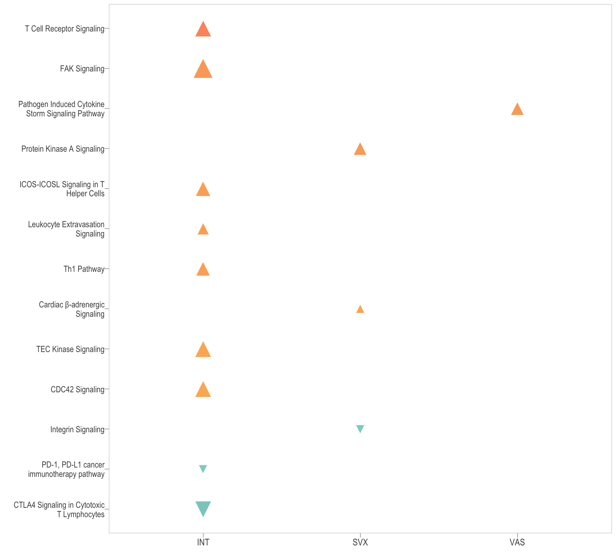
ggsave(filename = paste0("combine_ipa_dot.svg"), plot = path_dot1, path = here::here("2_plots/"),
       width = 11, height = 13, units = "cm")
Upstream Regulators
library(stringr)
upstream <- read_excel_allsheets(here::here("0_data/raw_data/IPA_upstreamRegs.xlsx"))

upstream <- lapply(upstream, function(x) {
  colnames(x) <- c("name", "exprLogRatio", "type", "activationState", "activationScore", "pval", "molecules", "network")
  x <- x %>% dplyr::mutate(logPval = -log10(pval), .after = pval)
  x$name <- x$name %>% firstCap() %>% str_wrap(width = 45)
  return(x)
})

# interesting_type <- c("cytokine", "group", "transmembrane receptor", "transcription regulator")
intersect_upstream <- intersect(upstream[[1]]$name,upstream[[2]]$name) %>% intersect(., upstream[[3]]$name)
# interesting_upstream <- c("beta-estradiol", "prednisolone", "PRL", "Tgf beta", "TGFB1", "FGF7", "BMP2", "FGF2", "VEGFA", "HIF1A")

heatMatrix_up <- lapply(upstream, function(x) {
  x <- x[!str_detect(x$type, "chemical"),]
  x <- bind_rows(
    x %>%
      dplyr::filter(activationScore > 0) %>%
      arrange(desc(logPval)) %>%
      head(18))
  x <- x %>% remove_rownames()
  mat <- x %>% dplyr::select(c("name", "activationScore", "type"))
  return(mat)
})

heatMatrix_down <- lapply(upstream, function(x) {
  x <- x[!str_detect(x$type, "chemical"),]
  x <- bind_rows(
    x %>%
      dplyr::filter(activationScore < 0) %>%
      arrange(desc(logPval)) %>%
      head(18))
  x <- x %>% remove_rownames()
  mat <- x %>% dplyr::select(c("name", "activationScore", "type"))
  return(mat)
})

heatMatrix_up <- merge(heatMatrix_up[[1]],heatMatrix_up[[2]],by= "name", all=T) %>% merge(.,heatMatrix_up[[3]],by= "name", all=T)
colnames(heatMatrix_up) <- c("name","INT", "type", "SVX", "type2", "VAS", "type3")
heatMatrix_up <- heatMatrix_up %>%
  dplyr::mutate(combinedType = coalesce(type, type2, type3)) %>%
  # dplyr::mutate(combinedType = factor(combinedType, levels = interesting_type)) %>%
  arrange(combinedType) %>% dplyr::select(c("name","INT", "SVX", "VAS", "combinedType"))
heatMatrix_up$name <- gsub("MiR-30c-5p \\(and other miRNAs w/seed GUAAACA\\)", "MiR-30c-5p", heatMatrix_up$name)

lookup <- tibble(gene_name = lm_all[[1]]$gene_name, gene_name_CAP = str_to_upper(lm_all[[1]]$gene_name))
replacement_vector <- setNames(lookup$gene_name, lookup$gene_name_CAP)
replacement_vector <- replacement_vector[!is.na(names(replacement_vector)) & names(replacement_vector) != ""]

# heatMatrix_up <- heatMatrix_up[[1]]
heatMatrix_up$correctName <- map_chr(heatMatrix_up$name, ~ str_replace_all(., replacement_vector))

heatMatrix_up$correctName <- str_replace_all(heatMatrix_up$correctName, ",", "/")

heatMatrix_up <- heatMatrix_up %>% filter(!is.na(INT))

# saveRDS(heatMatrix, here::here("0_data/rds_objects/heatMatrix.rds"))
# heatMatrix <- readRDS(here::here("0_data/rds_objects/heatMatrix.rds"))

heatMatrix_up_anno <- heatMatrix_up[,c(1,6)]

heatMatrix_up_anno <- heatMatrix_up_anno %>% left_join(lm_all[[2]][,c("gene_name","adj.P.Val")],by = join_by(correctName == gene_name)) %>% dplyr::rename(INT = adj.P.Val)

heatMatrix_up_anno <- heatMatrix_up_anno %>% left_join(lm_all[[3]][,c("gene_name","adj.P.Val")],by = join_by(correctName == gene_name)) %>% dplyr::rename(SVX = adj.P.Val)

heatMatrix_up_anno <- heatMatrix_up_anno %>% left_join(lm_all[[4]][,c("gene_name","adj.P.Val")],by = join_by(correctName == gene_name)) %>% dplyr::rename(VAS = adj.P.Val)

heatMatrix_up_anno <- heatMatrix_up_anno %>%
  dplyr::mutate(across(where(is.numeric), ~ as.character(signif(., 3)))) %>%
  dplyr::mutate(across(c(INT, SVX, VAS), ~ case_when(
    as.numeric(.) < 0.0001 ~ "****",
    as.numeric(.) < 0.001 ~ "***",
    as.numeric(.) < 0.01 ~ "**",
    as.numeric(.) < 0.05 ~ "*",
    TRUE ~ as.character(.)
  )))


heatMatrix_down <- merge(heatMatrix_down[[1]],heatMatrix_down[[2]],by= "name", all=T) %>% merge(.,heatMatrix_down[[3]],by= "name", all=T)
colnames(heatMatrix_down) <- c("name","INT", "type", "SVX", "type2", "VAS", "type3")
heatMatrix_down <- heatMatrix_down %>%
  dplyr::mutate(combinedType = coalesce(type, type2, type3)) %>%
  # dplyr::mutate(combinedType = factor(combinedType, levels = interesting_type)) %>%
  arrange(combinedType) %>% dplyr::select(c("name","INT", "SVX", "VAS", "combinedType"))
heatMatrix_down$name <- gsub("MiR-30c-5p \\(and other miRNAs w/seed GUAAACA\\)", "MiR-30c-5p", heatMatrix_down$name)

# heatMatrix_down <- heatMatrix_down[[1]]

heatMatrix_down$correctName <- map_chr(heatMatrix_down$name, ~ str_replace_all(., replacement_vector))

heatMatrix_down$correctName <- str_replace_all(heatMatrix_down$correctName, ",", "/")

heatMatrix_down <- heatMatrix_down %>% filter(!is.na(INT))

heatMatrix_down_anno <- heatMatrix_down[,c(1,6)]

heatMatrix_down_anno <- heatMatrix_down_anno %>% left_join(lm_all[[2]][,c("gene_name","adj.P.Val")],by = join_by(correctName == gene_name)) %>% dplyr::rename(INT = adj.P.Val)

heatMatrix_down_anno <- heatMatrix_down_anno %>% left_join(lm_all[[3]][,c("gene_name","adj.P.Val")],by = join_by(correctName == gene_name)) %>% dplyr::rename(SVX = adj.P.Val)

heatMatrix_down_anno <- heatMatrix_down_anno %>% left_join(lm_all[[4]][,c("gene_name","adj.P.Val")],by = join_by(correctName == gene_name)) %>% dplyr::rename(VAS = adj.P.Val)

heatMatrix_down_anno <- heatMatrix_down_anno %>%
  dplyr::mutate(across(where(is.numeric), ~ as.character(signif(., 3)))) %>%
  dplyr::mutate(across(c(INT, SVX, VAS), ~ case_when(
    as.numeric(.) < 0.0001 ~ "****",
    as.numeric(.) < 0.001 ~ "***",
    as.numeric(.) < 0.01 ~ "**",
    as.numeric(.) < 0.05 ~ "*",
    TRUE ~ as.character(.)
  )))


# df for heatmap annotation of sample group
anno <- dplyr::select(.data = rbind(heatMatrix_up, heatMatrix_down), c("name","combinedType"))
anno$combinedType <- str_to_title(anno$combinedType)
# anno <- anno[1:46,1:2] %>% column_to_rownames("name")
colnames(anno) <- c("name","Molecule Type")
anno$`Molecule Type` <- gsub("Transmembrane Receptor", "Transmembrane\nreceptor", anno$`Molecule Type`)
anno$`Molecule Type` <- gsub("Transcription Regulator", "Transcription\nregulator", anno$`Molecule Type`)
anno$`Molecule Type` <- gsub("Ligand-Dependent Nuclear Receptor", "Ligand-dependent\nnuclear receptor", anno$`Molecule Type`)
anno$`Molecule Type` <- gsub("G-Protein Coupled Receptor", "GPCRs", anno$`Molecule Type`)
anno$`Molecule Type` <- gsub("Mature Microrna", "Mature miRNA", anno$`Molecule Type`)
anno$`Molecule Type` <- gsub("Microrna", "miRNA", anno$`Molecule Type`)
anno$`Molecule Type` <- factor(anno$`Molecule Type`)
# colorRampPalette(rev(c("#FB8072","#FDB462","#ffffd5","#8DD3C7","#80B1D3")))(300)
anno_colours <- colorRampPalette(brewer.pal(9, "Set1"))(length(levels(anno$`Molecule Type`)))
names(anno_colours) <- levels(anno$`Molecule Type`)

mat1 <- heatMatrix_up[,c(1,2,3,4)] %>% column_to_rownames("name") %>% as.matrix()
mat1[is.na(mat1)] <- 0
mat1_anno <- heatMatrix_up_anno[,c(1,3,4,5)] %>% column_to_rownames("name") %>% as.matrix()
mat1_anno[is.na(mat1_anno)] <- ""


mat2 <- heatMatrix_down[,1:4] %>% remove_rownames() %>%  column_to_rownames("name") %>% as.matrix()
mat2[is.na(mat2)] <- 0
mat2_anno <- heatMatrix_down_anno[,c(1,3,4,5)] %>% remove_rownames() %>%  column_to_rownames("name") %>% as.matrix()
mat2_anno[is.na(mat2_anno)] <- ""

breaks <-seq(-3.5,3.5, by = 1)
#
# showtext_auto(enable = T)
hmap1 <- pheatmap(
      # MAIN
      mat = mat1,
      display_numbers = mat1_anno,
      color = colorRampPalette(rev(c("#FB8072","#FDB462","grey95","#8DD3C7","#80B1D3")))(length(breaks)),
      cellwidth = 35,
      # cellheight = 40,
      scale = "none",

      # Col
      cluster_cols = F,
      border_color = "white",
      angle_col = "0",
      # gaps_row = c(23,30,38),

      # Row
      cluster_rows = F,

      # Labs
      show_colnames = T,
      show_rownames = T,
      legend = F,
      breaks = breaks,
      heatmap_legend_param = list(title = "Z-score", legend_width = unit(7, "cm")),

      # Annotation
      annotation_legend = F,
      # legend_labels = T,
      annotation_row = anno[anno$name %in% rownames(mat1),1:2] %>% remove_rownames() %>% column_to_rownames("name"),
      annotation_colors = list("Molecule Type" = anno_colours),

      annotation_names_row = F,

      # Fonts
      fontfamily = "Arial",
      fontsize = 12,
      fontsize_col = 12,
      fontsize_number = 8,
      fontsize_row = 10

    ) %>% as.ggplot()

hmap2 <- pheatmap(
      # MAIN
      mat = mat2,
      display_numbers = mat2_anno,
      color = colorRampPalette(rev(c("#FB8072","#FDB462","grey95","#8DD3C7","#80B1D3")))(length(breaks)),
      cellwidth = 35,
      # cellheight = 40,
      scale = "none",

      # Col
      cluster_cols = F,
      border_color = "white",
      angle_col = "0",

      # Row
      cluster_rows = F,

      # Labs
      show_colnames = T,
      show_rownames = T,
      legend = T,
      breaks = breaks,
      # heatmap_legend_param = list(title = "Z-score", legend_width = unit(7, "cm")),
      heatmap_legend_param = list(title = "Z-score",
                                  direction= "vertical",
                                  merge_legend = T,
                                  legend_direction = "vertical",
                                  legend_height = unit(4, "cm")),
      # Annotation
      annotation_legend = T,
      # legend_labels = T,
      annotation_row = anno[anno$name %in% rownames(mat2),1:2] %>% remove_rownames() %>% column_to_rownames("name"),
      annotation_colors = list("Molecule Type" = anno_colours),

      annotation_names_row = F,

      # Fonts
      fontfamily = "Arial",
      fontsize = 12,
      fontsize_col = 12,
      fontsize_number = 8,
      fontsize_row = 10

    ) %>% as.ggplot()


# png(filename = here::here("2_plots/3_FA/ipa/legend.png"),res = 900,width = 8.267,height = 10.63,units = "in")
# draw(hmap2, merge_legend = T, heatmap_legend_side = "right",
#      annotation_legend_side = "right")
# dev.off()

hmap_combined <- hmap1 + plot_spacer() + hmap2 +
  plot_layout(widths = c(4,-1.2,4.5))

hmap_combined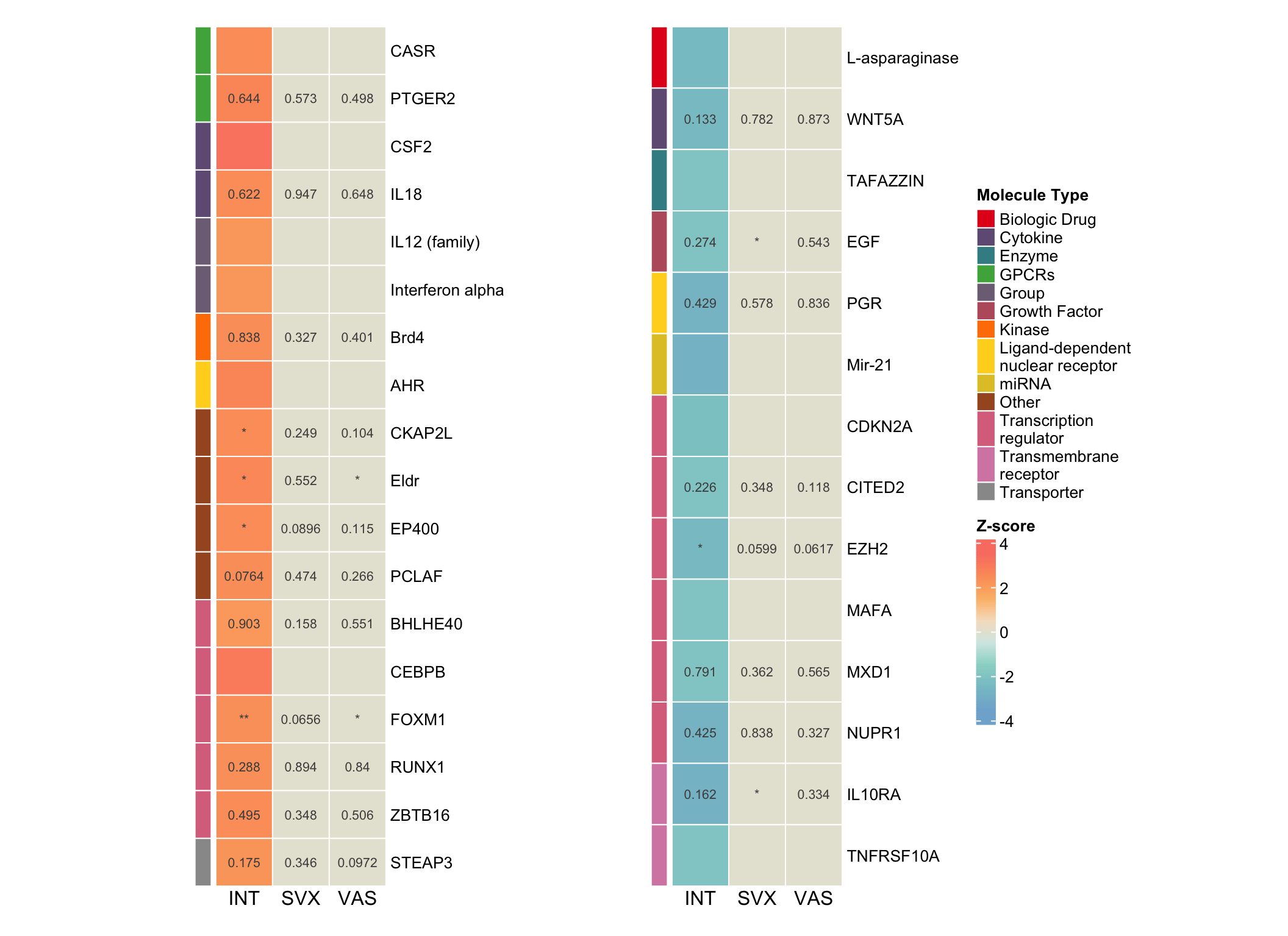
ggsave(filename = "upstream_hmap.svg", plot = hmap_combined, path = here::here("2_plots/"),
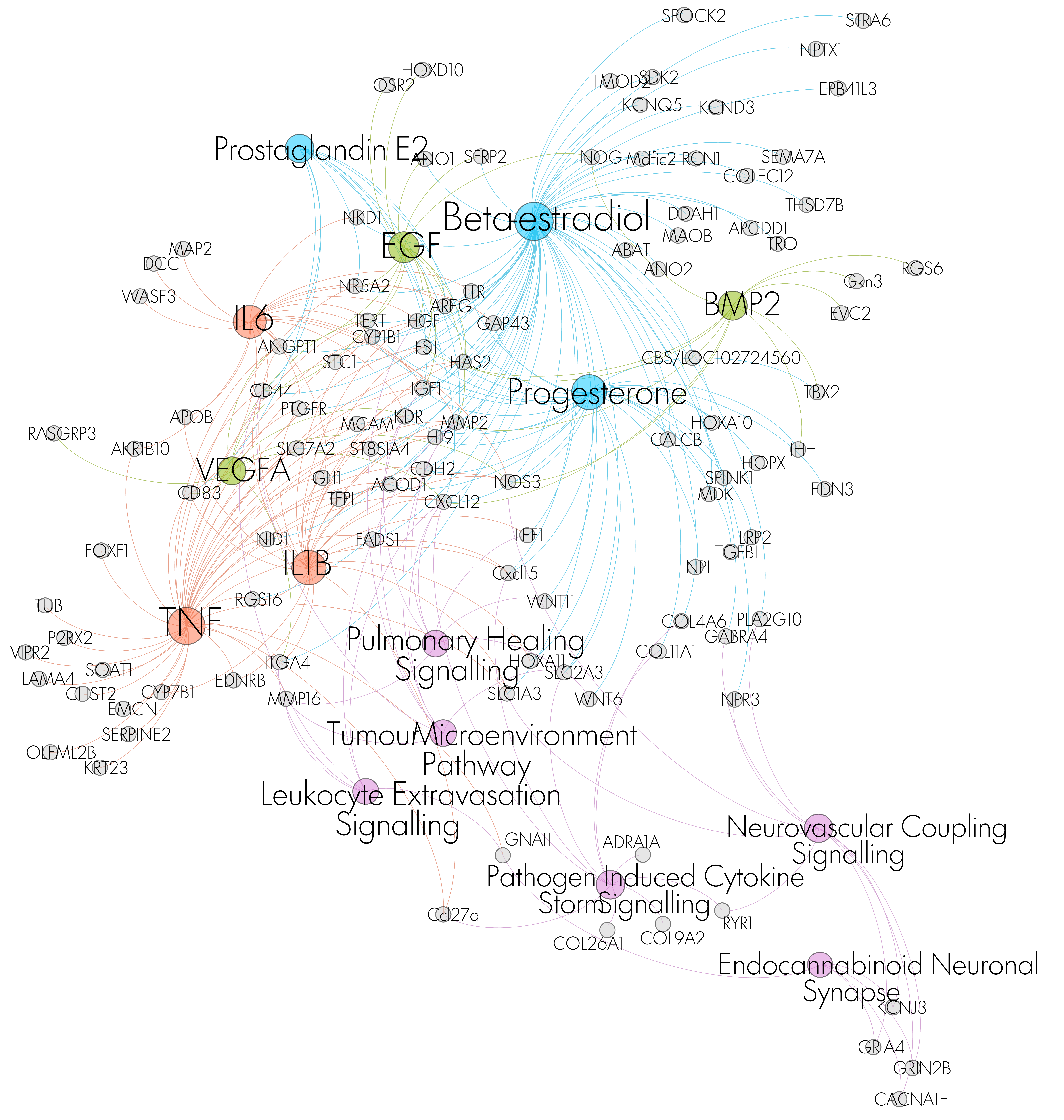
width = 18, height = 11, units = "cm")Disease and Function
disease_function <- read_excel_allsheets(here::here("0_data/raw_data/IPA_disease_function.xlsx"))
disease_function <- lapply(disease_function, function(x) {
  colnames(x) <- c("Categories", "name", "pval", "activationState", "activationScore", "molecules", "numMolecules")
  x <- x %>% separate(col = Categories, sep = ",", into = c("Category 1", "Category 2", "Category 3",
                                                            "Category 4", "Category 5", "Category 6",
                                                            "Category 7", "Category 8", "Category 9",
                                                            "Category 10", "Category 11"),remove = F,fill = "right")
  x <- x %>% dplyr::mutate(logPval = -log10(pval), .after = pval)
  # x$name <- x$name %>% firstCap() %>% str_wrap(width = 45)
  return(x)
})

library(stringr)
dnf_terms <- disease_function[[1]] %>% slice(.,1:50) %>% arrange(desc(logPval))  %>%  separate_rows(data = ., molecules, sep = ",")
dnf_terms$`Category 1` <- dnf_terms$`Category 1` %>% str_to_upper()
dnf_terms$name <- dnf_terms$name %>% firstCap() %>% str_wrap(width = 45)

# Load libraries
library(ggraph)
library(igraph)
library(tidyverse)
library(RColorBrewer)
# library(dplyr)

# Step 1: Define edges to represent the hierarchy
edges_t <- dnf_terms %>%
  arrange(`Category 1`, name) %>%
  select(Category_1 = `Category 1`, name) %>%
  distinct() %>%
  dplyr::rename(.,from = Category_1, to = name)

t <- data.frame(from = "origin", to = unique(edges_t$from))

edges_t <- rbind(t, edges_t)

connect_t <- dnf_terms %>%
  arrange(`Category 1`, name) %>%
  select(name, molecules) %>%
  # separate_rows(molecules, sep = ",") %>%
  group_by(molecules) %>%
  filter(n() > 1) %>%  # Retain only molecules appearing in multiple "name" entries
  reframe(connections = combn(name, 2, simplify = FALSE)) %>%
  unnest_wider(connections, names_sep = "_") %>%
  dplyr::rename(from = connections_1, to = connections_2)
connect_t$value <- runif(nrow(connect_t)) ###

# Condense connect_t by removing 'molecules', counting unique connections, and removing reciprocal pairs
connect_t <- connect_t %>%
  # select(-molecules) %>%                  # Remove the 'molecules' column
  mutate(pair = map2_chr(from, to, ~paste(sort(c(.x, .y)), collapse = "-"))) %>% # Create unique identifier for pairs
  group_by(pair) %>%                      # Group by the unique 'from'-'to' pairs
  summarise(from = first(from),            # Retain the original 'from' and 'to' values
            to = first(to),
            value = n(), .groups = "drop") %>%  # Count occurrences to represent the number of molecules between pairs
  dplyr::select(-pair)                           # Remove the 'pair' column after processing


# Step 3: Create a vertices data frame
vertices_t <- tibble(
  name = unique(c(edges_t$from, edges_t$to)),
  # group = if_else(name %in% edges_t$from, NA_character_, edges_t$from[match(name, edges_t$to)]),
)

# Let's add a column with the group of each name. It will be useful later to color points
vertices_t$group  <-  edges_t$from[ match( vertices_t$name, edges_t$to ) ]

# Add 'value' after ensuring vertices_t is fully initialized
vertices_t$value <- dnf_terms$numMolecules[ match( vertices_t$name, dnf_terms$name) ]

vertices_t$state <- dnf_terms$activationState[ match( vertices_t$name, dnf_terms$name) ]


# Calculate angle and position for labels
vertices_t$id <- NA
myleaves <- which(is.na(match(vertices_t$name, edges_t$from)))
nleaves <- length(myleaves)
vertices_t$id[myleaves] <- seq(1:nleaves)
vertices_t$angle <- 90 - 360 * (vertices_t$id / nleaves)

# Calculate label alignment and angle adjustment
vertices_t$hjust <- ifelse(vertices_t$angle < -90, 1, 0)
vertices_t$angle <- ifelse(vertices_t$angle < -90, vertices_t$angle + 180, vertices_t$angle)

# Step 4: Create the graph
mygraph_t <- graph_from_data_frame(edges_t, vertices = vertices_t)

# Match connections to vertex IDs
from_t <- match(connect_t$from, vertices_t$name)
to_t <- match(connect_t$to, vertices_t$name)

# Step 5: Create the plot
dnf_plot <- ggraph(mygraph_t, layout = 'dendrogram', circular = T) +
  geom_conn_bundle(data = get_con(from = from_t, to = to_t),aes(colour=..index..), edge_alpha = 0.5,edge_width = 0.5, tension = 1) +
  scale_edge_colour_distiller(palette = "Greys") +

  # Adjust label positions and colors for better separation
  geom_node_text(aes(x = x*1.3, y = y*1.3, label = name, angle = angle, hjust = hjust, colour = group), size = 4, alpha = 1,show.legend = F) +

  # Add node points for clarity
   geom_node_point(aes(filter = leaf, x = x*1.1, y=y*1.1, colour=group, size=value, alpha=0.2)) +
  scale_colour_manual(values = colorRampPalette(brewer.pal(10, "Paired"))(13)) +
  # scale_shape_manual(values = c(15, 16),) +
  scale_size(range = c(5,18),limits = c(min(dnf_terms$numMolecules), max(dnf_terms$numMolecules)) ) +
  theme_void() +
  theme(
    legend.position = "none",
    plot.margin = unit(c(0, 0, 0, 0), "cm")
  ) +
  expand_limits(x = c(-3, 3), y = c(-3, 3))

ggsave(filename = "dnf_plot.svg", plot = dnf_plot,path = here::here("2_plots/"),width = 40, height = 40, units = "cm")
# wrap_plots(list(combine_ipaPath, dnf_plot))
#
dnf_plot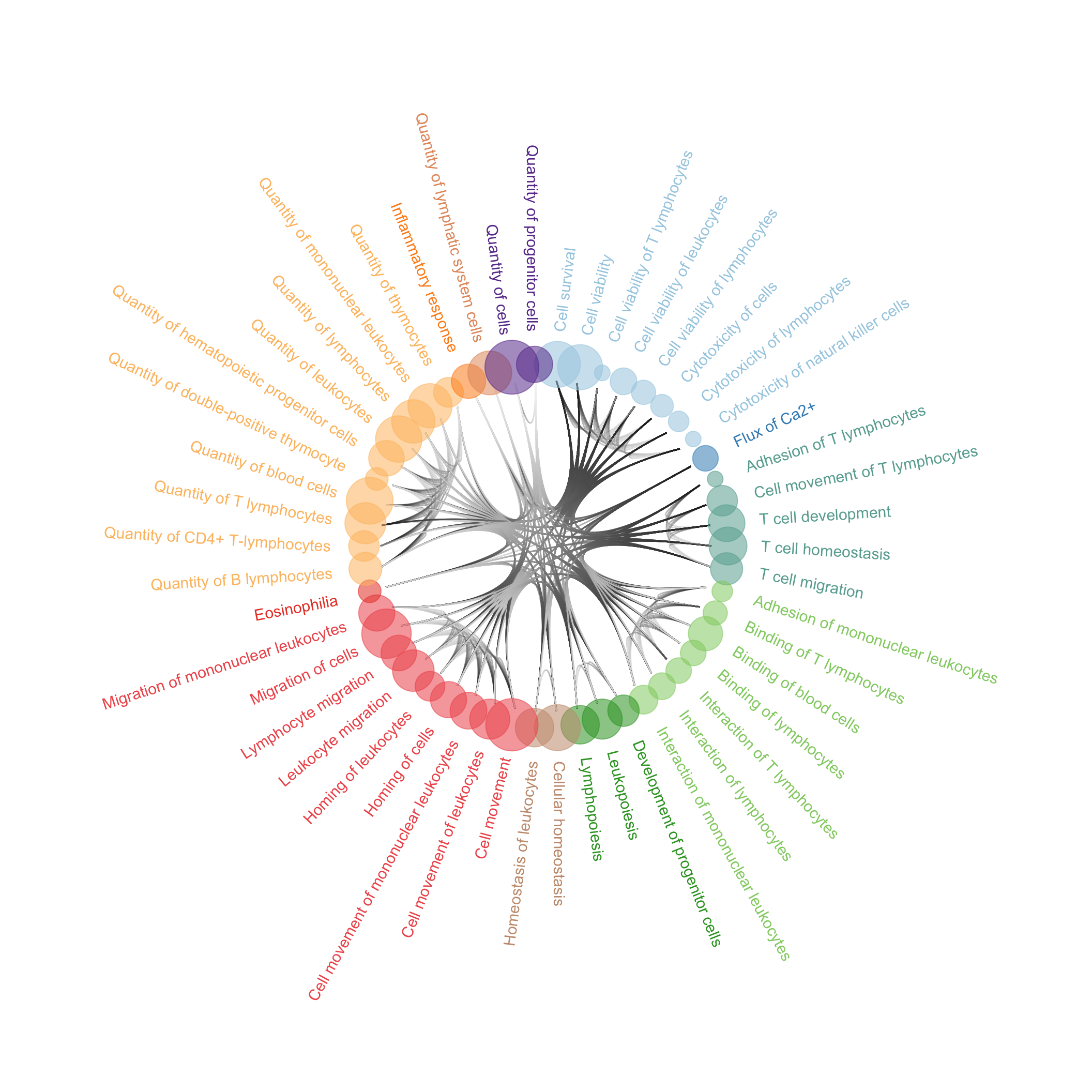
| Version | Author | Date |
|---|---|---|
| 5dce909 | Ha Tran | 2024-11-07 |
INT vs CONT
Network plot
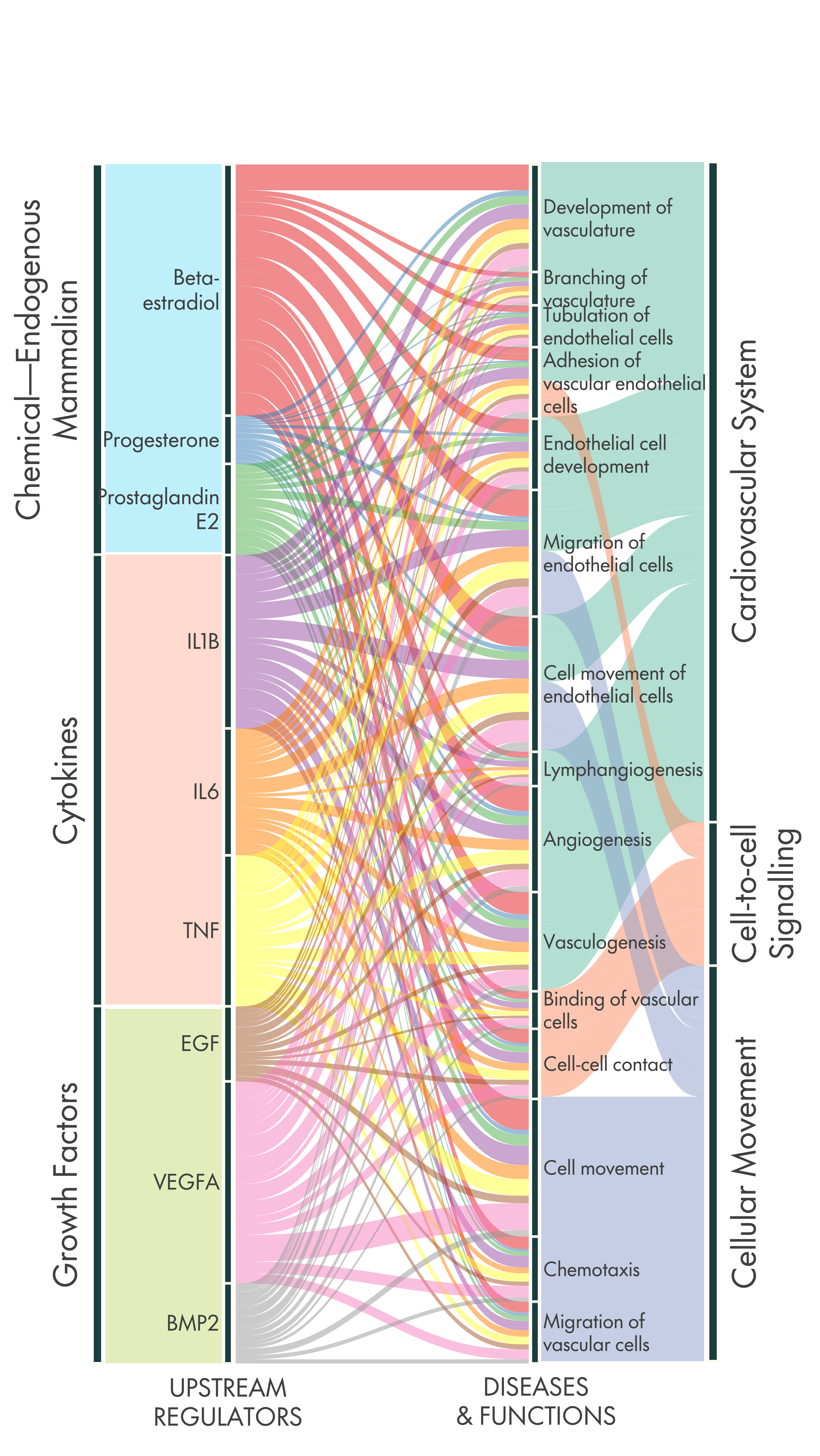
Alluvial plot
Extra figures
Supp Fig 1
patch <- readRDS(here::here("0_data/functions/patch.rds"))
enrichGO_sig <- readRDS(here::here("0_data/RDS_objects/enrichGO_sig_new.rds"))

collatedPath <- read_excel_allsheets(here::here("0_data/raw_data/Immune-related enriched terms GO Kegg reactome KF_15102024.xlsx"))

collatedPath <- collatedPath$`Collated - all databases` %>%
  dplyr::filter(if_any(c(`Signigifcant in comparison`, Also, `Also 2`), ~ . == "INT vs SVX/VAS")) %>% dplyr::mutate(`Pathway description` = `Pathway description`%>% firstCap() %>% str_wrap(width = 45))

go <- collatedPath %>% filter(str_detect(Database,"GO")) %>%
  dplyr::filter(`Pathway description` %in% enrichGO_sig$`INT vs SVX_VAS`$Description)

# combine all df in list into one df
go_dot_all <- as.data.frame(do.call(rbind, enrichGO_sig[c(2,3,4)])) %>%
  rownames_to_column("group") %>%
  dplyr::filter(Description %in% go$`Pathway description`)

# clean group names and change to factor
go_dot_all$group <- gsub(pattern = "\\..*", "", go_dot_all$group) %>% as.factor()

# go_subset <- lapply(enrichGO_sig, function(x) { x %>% filter(Description %in% go_dot_all$Description)})
# factor the descriptions

top <- as.data.frame(do.call(rbind, lapply(enrichGO_sig[c(2, 3, 4)], function(x) {
  x %>% dplyr::filter(Description %in% go_dot_all$Description) %>%
    arrange(p.adjust) %>%
    dplyr::slice(1:40) %>%
    dplyr::select(3)
}))) %>% rownames_to_column("group")

top <- melt(top, "group")

terms <- top$value %>% as.factor() %>% levels()
go_dot_all <- go_dot_all[go_dot_all$Description %in% terms,]
go_dot_all$group <- gsub(pattern = " vs SVX_VAS", "", go_dot_all$group) %>% as.factor()
go_dot_all$group <- factor(go_dot_all$group,levels = c("INT", "SVX", "VAS"))
go_dot_all$Description <- go_dot_all$Description %>% str_wrap(38)
combine_go_1 <- ggplot(go_dot_all[1:25,]) +
  geom_point(aes(x = group, y = reorder(Description, logFDR), colour = logFDR, size = Count, shape = ONTOLOGY %>% as.factor())) +
  scale_color_gradientn(colors = rev(c("#FB8072","#FDB462","#8DD3C7","#80B1D3")),
                        values = scales::rescale(c(min(go_dot_all$logFDR), max(go_dot_all$logFDR))),
                        limits = c(min(go_dot_all$logFDR), max(go_dot_all$logFDR)),
                        breaks = scales::pretty_breaks(n = 5)) +
  scale_x_discrete(drop = F)+
  scale_size(range = c(2,8), limits = c(min(go_dot_all$Count), max(go_dot_all$Count))) +
  labs(x = "", y = "", color = expression("-log"[10] * "FDR"), size = "Counts", shape = "Ontology")+
  bossTheme(base_size = 14,legend = "right")

combine_go_2 <- ggplot(go_dot_all[26:62,]) +
  geom_point(aes(x = group, y = reorder(Description, logFDR), colour = logFDR, size = Count, shape = ONTOLOGY %>% as.factor())) +
  scale_color_gradientn(colors = rev(c("#FB8072","#FDB462","#8DD3C7","#80B1D3")),
                        values = scales::rescale(c(min(go_dot_all$logFDR), max(go_dot_all$logFDR))),
                        limits = c(min(go_dot_all$logFDR), max(go_dot_all$logFDR)),
                        breaks = scales::pretty_breaks(n = 5)) +
  scale_x_discrete(drop = F)+
  scale_size(range = c(2,8), limits = c(min(go_dot_all$Count), max(go_dot_all$Count))) +
  labs(x = "", y = "", color = expression("-log"[10] * "FDR"), size = "Counts", shape = "Ontology")+
  bossTheme(base_size = 14,legend = "right")

combine_go <- list(combine_go_1,combine_go_2) %>% patch(.,legend = "bottom")

# if(savePlots == TRUE) {
#   ggsave(filename = paste0("immune_go.svg"), plot = combine_go, path = here::here("2_plots/4_paper"), width = 20, height = 25, units = "cm")
# }


combine_go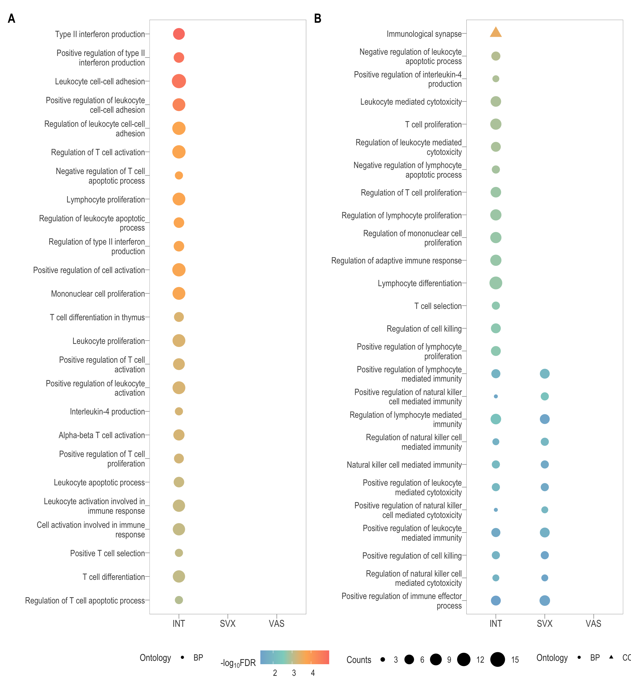
| Version | Author | Date |
|---|---|---|
| d519e7f | Ha Tran | 2024-12-03 |
# ggsave(filename = paste0("immune_go.svg"), plot = combine_go, path = here::here("2_plots/4_paper"), width = 33, height = 45, units = "cm")Supp Fig 2
enrichKEGG_sig <- readRDS(here::here("0_data/RDS_objects/enrichKEGG_sig.rds"))

# combine all df in list into one df
kegg_dot_all <- as.data.frame(do.call(rbind, enrichKEGG_sig[c(2,3,4)])) %>%
  rownames_to_column("group")
# kegg_dot_all <- kegg_dot_all[! kegg_dot_all$group %in% c("DT+Treg vs veh"),]
# clean group names and change to factor
kegg_dot_all$group <- gsub(pattern = "\\..*", "", kegg_dot_all$group) %>% as.factor()
kegg_dot_all$group <- gsub(pattern = " vs SVX_VAS", "", kegg_dot_all$group) %>% as.factor()
kegg_dot_all$group <- factor(kegg_dot_all$group, levels = c("INT", "SVX", "VAS"))
# kegg_dot_all$group <- factor(kegg_dot_all$group,levels = c("DT vs veh", "DT+Treg vs veh", "DT+Treg vs DT" ))
kegg_dot_all$Description <- kegg_dot_all$Description %>% str_wrap(38)
combine_kegg <- ggplot(kegg_dot_all) +
  geom_point(aes(x = group, y = reorder(Description, logFDR), colour = logFDR, size = Count)) +
  scale_color_gradientn(colors = rev(c("#FB8072","#FDB462","#8DD3C7","#80B1D3")),
                        values = scales::rescale(c(min(kegg_dot_all$logFDR), max(kegg_dot_all$logFDR))),
                        breaks = scales::pretty_breaks(n = 5)) +
  scale_x_discrete(drop = F)+
  scale_size(range = c(2,8),limits = c(2, 11)) +
  labs(x = "", y = "", color = expression("-log"[10] * "FDR"), size = "Counts")+
  bossTheme(base_size = 14,legend = "right")


if(savePlots == TRUE) {
  ggsave(filename = paste0("combine_kegg_dot.svg"), plot = combine_kegg, path = here::here("2_plots/3_FA/kegg/"),
         width = 18, height = 20, units = "cm")
}


# combine_kegg
reactome_sig <- readRDS(here::here("0_data/RDS_objects/reactome_sig.rds"))
react <- collatedPath %>% filter(str_detect(Database,"Reactome")) %>%
filter(`Pathway description` %in% reactome_sig$`INT vs SVX_VAS`$Description)
# combine all df in list into one df
react_dot_all <- as.data.frame(do.call(rbind, reactome_sig[c(2,3,4)])) %>%
rownames_to_column("group") %>%
filter(Description %in% react$`Pathway description`)
# clean group names and change to factor
react_dot_all$group <- gsub(pattern = "\\..*", "", react_dot_all$group) %>% as.factor()
# react_subset <- lapply(reactome_sig, function(x) { x %>% filter(Description %in% react_dot_all$Description)})
# factor the descriptions
top <- do.call(rbind, lapply(reactome_sig[c(2, 3, 4)], function(x) {
x %>% as.data.frame() %>%
filter(Description %in% react_dot_all$Description) %>%
arrange(p.adjust) %>%
dplyr::select(1)
})) %>% rownames_to_column("group")
top <- melt(top, "group")
terms <- top$value %>% as.factor() %>% levels()
react_dot_all <- react_dot_all[react_dot_all$Description %in% terms,]
react_dot_all$group <- gsub(pattern = " vs SVX_VAS", "", react_dot_all$group) %>% as.factor()
react_dot_all$group <- factor(react_dot_all$group,levels = c("INT", "SVX", "VAS"))
react_dot_all$Description <- react_dot_all$Description %>% str_wrap(38)
combine_react <- ggplot(react_dot_all) +
geom_point(aes(x = group, y = reorder(Description, logFDR), colour = logFDR, size = Count)) +
scale_color_gradientn(colors = rev(c("#FB8072","#FDB462","#8DD3C7","#80B1D3")),
values = scales::rescale(c(min(react_dot_all$logFDR), max(react_dot_all$logFDR))),
limits = c(min(react_dot_all$logFDR), max(react_dot_all$logFDR)),
breaks = scales::pretty_breaks(n = 5)) +
scale_x_discrete(drop = F)+
scale_size(range = c(2,8), limits = c(2,11)) +
labs(x = "", y = "", color = expression("-log"[10] * "P value"), size = "Counts")+
bossTheme(base_size = 14,legend = "right")
# combine_react
# if(savePlots == TRUE) {
# ggsave(filename = paste0("immune_react.svg"), plot = combine_react, path = here::here("2_plots/4_paper"), width = 20, height = 25, units = "cm")
# }
# ggsave(filename = paste0("immune_react.svg"), plot = combine_react, path = here::here("2_plots/4_paper"), width = 33, height = 45, units = "cm")vol <- readRDS(here::here("0_data/RDS_plots/vol_plots.rds"))
patch(list(combine_kegg, combine_react),ncol = 2) 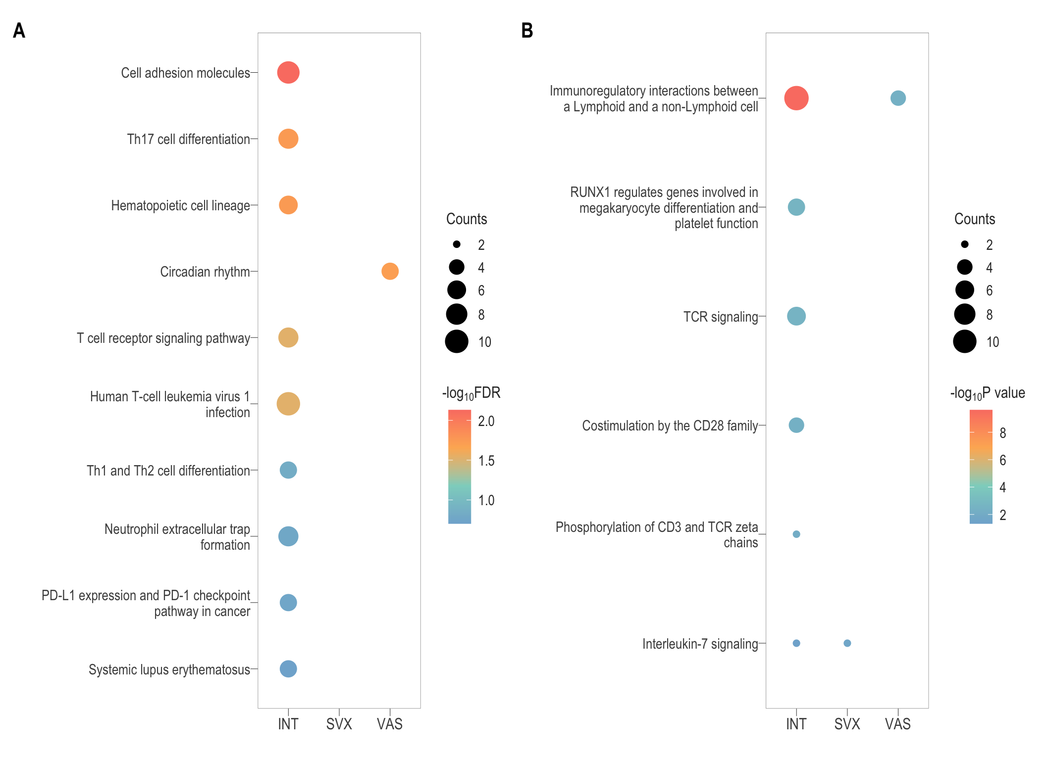
| Version | Author | Date |
|---|---|---|
| d519e7f | Ha Tran | 2024-12-03 |
# %>% ggsave(plot = .,filename = "kegg_react.svg", path = here::here("2_plots/4_paper/"), width = 33, height = 15, units = "cm")

design = "
AABB
CCDD
CCDD
"

patch(list(vol[[3]], vol[[4]]),ncol = 2)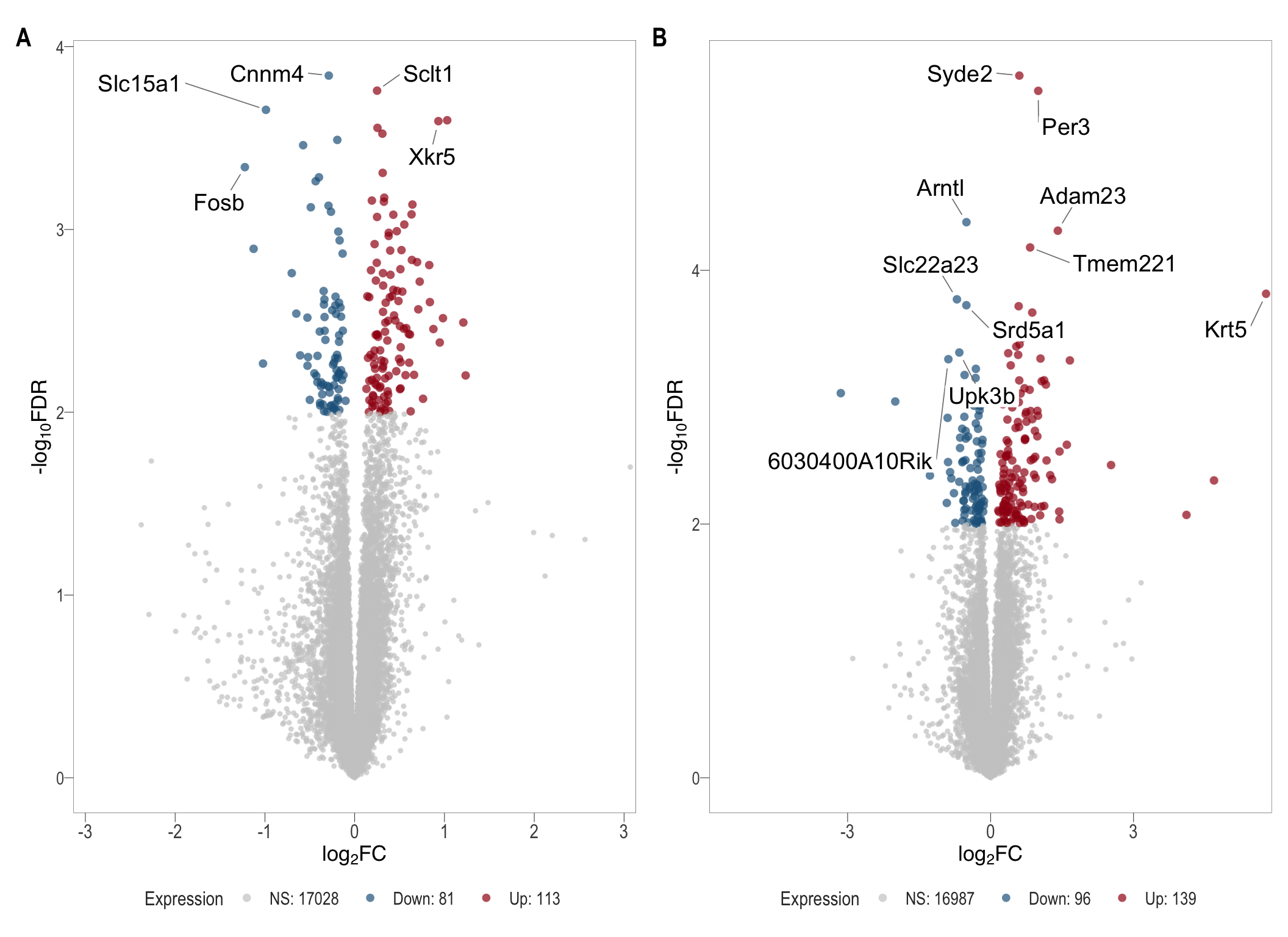
| Version | Author | Date |
|---|---|---|
| d519e7f | Ha Tran | 2024-12-03 |
# %>% ggsave(plot = .,filename = "volcanos.svg", path = here::here("2_plots/4_paper/"), width = 33, height = 30, units = "cm")

# ggsave(plot = vol[[3]] + theme(legend.position = "right"),filename = "volcano_SVX.svg", path = here::here("2_plots/4_paper/"), width = 11, height = 11, units = "cm")
# ggsave(plot = vol[[4]] + theme(legend.position = "right"),filename = "volcano_VAS.svg", path = here::here("2_plots/4_paper/"), width = 11, height = 11, units = "cm")
Fig 2
genes <- c("Trdc", "Trgc1", "Cd3e", "Trbc2", "Cd3g",
           "Lat", "Itk", "Grap2", "Blk", "Cd226", "Prkcq", "Havcr2", "Rasgrp1", "Itgal", "Btla",
           "Scart1", "Rorc", "Irf4",
           "Cxcr6", "Cxcr3", "Sell",
           "Il7r", "Il12rb1", "Il18rap")

degs <- do.call(rbind, lapply(lm_all[c(2,3,4)], function(x){
  x %>% as.data.frame() %>%
    dplyr::select(c("gene_name","logFC","AveExpr","description", "P.Value","adj.P.Val","entrezid","expression")) %>%
    dplyr::filter(gene_name %in% genes)
})) %>% rownames_to_column("group")


degs$group <- gsub(pattern = "\\..*", "", degs$group) %>% as.factor()
degs$group <- gsub(pattern = " vs SVX_VAS", "", degs$group) %>% as.factor()
degs$group <- factor(degs$group, levels = c("INT", "SVX", "VAS"))

degs_mat <- degs %>% dplyr::select(c("gene_name", "group", "logFC")) %>% dplyr::arrange(factor(gene_name, levels = genes)) %>%
  pivot_wider(.,names_from = "group", values_from = "logFC")  %>% column_to_rownames("gene_name")

degs_anno <- degs %>% dplyr::select(c("gene_name", "group", "adj.P.Val")) %>% dplyr::arrange(factor(gene_name, levels = genes)) %>%
  pivot_wider(.,names_from = "group", values_from = "adj.P.Val")  %>% column_to_rownames("gene_name") %>%
  dplyr::mutate(across(where(is.numeric), ~ as.character(signif(., 3)))) %>%
  dplyr::mutate(across(c(INT, SVX, VAS), ~ case_when(
    as.numeric(.) < 0.00001 ~ "****",
    as.numeric(.) < 0.0001 ~ "***",
    as.numeric(.) < 0.001 ~ "**",
    as.numeric(.) < 0.01 ~ "*",
    TRUE ~ as.character(.)
  )))


anno_degs <- tibble("name" = rownames(degs_mat), "Annotation" = c(rep("TCR complex", 5),
                                                                  rep("TCR signaling", 10),
                                                                  rep("Lymphocyte\ndifferentiation/\nmaturation", 3),
                                                                  rep("Cell homing\nand migration", 3),
                                                                  rep("Cytokine signaling", 3))) %>%
  dplyr::mutate(Annotation = factor(Annotation, levels = c("TCR complex",
                                                           "TCR signaling",
                                                           "Lymphocyte\ndifferentiation/\nmaturation",
                                                           "Cell homing\nand migration",
                                                           "Cytokine signaling")))
# colorRampPalette(rev(c("#FB8072","#FDB462","#ffffd5","#8DD3C7","#80B1D3")))(300)
anno_colours <- colorRampPalette(brewer.pal(5, "Set1"))(length(levels(anno_degs$Annotation)))
names(anno_colours) <- levels(anno_degs$Annotation)


degs_plot <- ComplexHeatmap::pheatmap(
    mat = degs_mat %>% as.matrix(),
    color = colorRampPalette(rev(c("#FB8072","#FDB462","#ffffd5","#8DD3C7","#80B1D3")))(300),
    scale = "row",
    display_numbers = degs_anno %>% as.matrix(),
    cluster_cols = F,
    border_color = "white",
    show_colnames = T,
    cluster_rows = F,
    gaps_col = c(1,2),
    gaps_row = c(5,15,18,21),
    legend = T,

    heatmap_legend_param = list(title = "Fold change Z-score",
                                direction= "horizontal",
                                merge_legend = T,
                                legend_direction = "horizontal",
                                legend_width = unit(5, "cm")),
    # Annotation
    annotation_legend = F,
    # legend_labels = T,
    annotation_row = anno_degs %>% remove_rownames() %>% column_to_rownames("name"),
    annotation_colors = list("Annotation" = anno_colours),

    annotation_names_row = F,
    # annotation_legend_param = list(direction = "horizontal"),

    fontfamily = "Arial",
    fontsize = 12,
    fontsize_col = 12,
    fontsize_number = 12,
    fontsize_row = 12, angle_col = "0",
    labels_row = as.expression(lapply(rownames(degs_mat), function(a) bquote(italic(.(a)))))
  ) %>% as.ggplot()

ggsave(plot = degs_plot ,filename = "subset_degs.svg", path = here::here("2_plots/4_paper/"), width = 18, height = 25, units = "cm")

degs_plot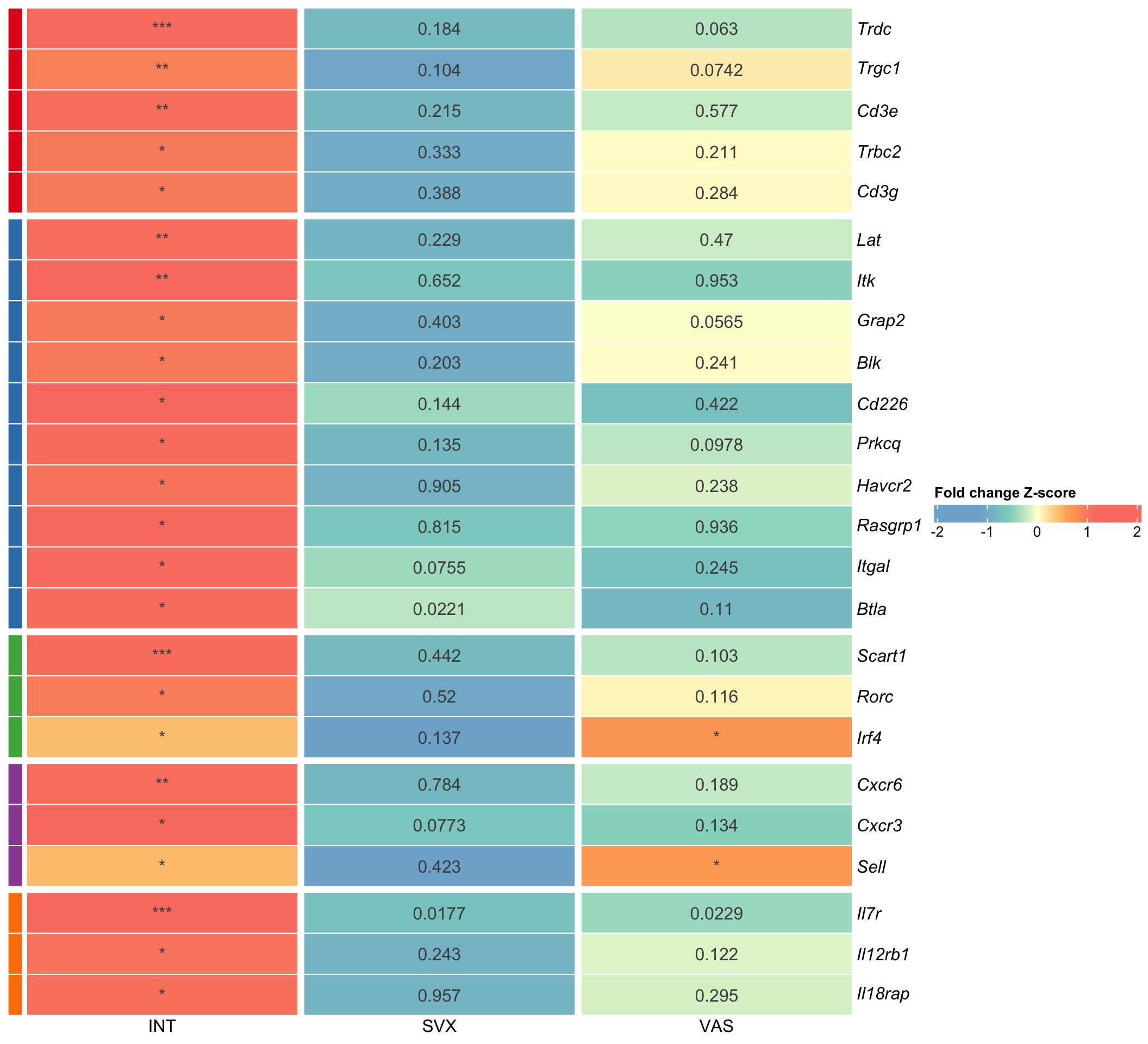
| Version | Author | Date |
|---|---|---|
| d519e7f | Ha Tran | 2024-12-03 |
# draw(degs_plot, merge_legend = F, heatmap_legend_side = "bottom", annotation_legend_side = "right" )

# if (savePlots == T) {
#   svg(filename = here::here("../2_plots/4_paper/selected_degs.svg"),width = 18,height = 25)
#   draw(heat_combined, merge_legend = T, heatmap_legend_side = "bottom",
#        annotation_legend_side = "bottom")
#   dev.off()
#   }
sessionInfo()R version 4.4.1 (2024-06-14)
Platform: aarch64-apple-darwin20
Running under: macOS 26.1
Matrix products: default
BLAS: /Library/Frameworks/R.framework/Versions/4.4-arm64/Resources/lib/libRblas.0.dylib
LAPACK: /Library/Frameworks/R.framework/Versions/4.4-arm64/Resources/lib/libRlapack.dylib; LAPACK version 3.12.0
locale:
[1] en_US.UTF-8/en_US.UTF-8/en_US.UTF-8/C/en_US.UTF-8/en_US.UTF-8
time zone: Australia/Adelaide
tzcode source: internal
attached base packages:
[1] grid stats graphics grDevices utils datasets methods
[8] base
other attached packages:
[1] ggraph_2.2.2 stringi_1.8.7 knitr_1.50
[4] pandoc_0.2.0 ggrepel_0.9.6 ggbiplot_0.6.2
[7] ggplotify_0.1.3 RColorBrewer_1.1-3 ggalluvial_0.12.5
[10] igraph_2.1.4 viridis_0.6.5 viridisLite_0.4.2
[13] cowplot_1.2.0 pander_0.6.6 kableExtra_1.4.0
[16] VennDiagram_1.7.3 futile.logger_1.4.3 patchwork_1.3.2
[19] readxl_1.4.5 extrafont_0.19 DT_0.34.0
[22] ComplexHeatmap_2.22.0 pheatmap_1.0.13 lubridate_1.9.4
[25] forcats_1.0.0 stringr_1.5.2 dplyr_1.1.4
[28] purrr_1.1.0 tidyr_1.3.1 ggplot2_4.0.0
[31] tidyverse_2.0.0 reshape2_1.4.4 tibble_3.3.0
[34] readr_2.1.5 magrittr_2.0.4 showtext_0.9-7
[37] showtextdb_3.0 sysfonts_0.8.9
loaded via a namespace (and not attached):
[1] gridExtra_2.3 formatR_1.14 rlang_1.1.6
[4] clue_0.3-66 GetoptLong_1.0.5 git2r_0.36.2
[7] matrixStats_1.5.0 compiler_4.4.1 png_0.1-8
[10] systemfonts_1.2.3 vctrs_0.6.5 pkgconfig_2.0.3
[13] shape_1.4.6.1 crayon_1.5.3 fastmap_1.2.0
[16] magick_2.9.0 labeling_0.4.3 promises_1.3.3
[19] rmarkdown_2.29 tzdb_0.5.0 ggbeeswarm_0.7.2
[22] ragg_1.5.0 xfun_0.53 cachem_1.1.0
[25] jsonlite_2.0.0 later_1.4.4 tweenr_2.0.3
[28] parallel_4.4.1 cluster_2.1.8.1 R6_2.6.1
[31] bslib_0.9.0 extrafontdb_1.0 jquerylib_0.1.4
[34] cellranger_1.1.0 Rcpp_1.1.0 iterators_1.0.14
[37] IRanges_2.40.1 httpuv_1.6.16 timechange_0.3.0
[40] tidyselect_1.2.1 rstudioapi_0.17.1 yaml_2.3.10
[43] doParallel_1.0.17 codetools_0.2-20 plyr_1.8.9
[46] withr_3.0.2 S7_0.2.0 ggrastr_1.0.2
[49] evaluate_1.0.5 gridGraphics_0.5-1 lambda.r_1.2.4
[52] polyclip_1.10-7 xml2_1.4.0 circlize_0.4.16
[55] pillar_1.11.1 whisker_0.4.1 foreach_1.5.2
[58] stats4_4.4.1 generics_0.1.4 rprojroot_2.1.1
[61] S4Vectors_0.44.0 hms_1.1.3 scales_1.4.0
[64] glue_1.8.0 tools_4.4.1 graphlayouts_1.2.2
[67] fs_1.6.6 tidygraph_1.3.1 Cairo_1.6-5
[70] Rttf2pt1_1.3.12 colorspace_2.1-1 beeswarm_0.4.0
[73] ggforce_0.5.0 vipor_0.4.7 cli_3.6.5
[76] rappdirs_0.3.3 textshaping_1.0.3 workflowr_1.7.2
[79] futile.options_1.0.1 svglite_2.2.1 gtable_0.3.6
[82] yulab.utils_0.2.1 sass_0.4.10 digest_0.6.37
[85] BiocGenerics_0.52.0 rjson_0.2.23 htmlwidgets_1.6.4
[88] farver_2.1.2 memoise_2.0.1 htmltools_0.5.8.1
[91] lifecycle_1.0.4 here_1.0.2 GlobalOptions_0.1.2
[94] MASS_7.3-65