KEGG Analysis
Ha M. Tran
22/08/2021
Last updated: 2023-09-16
Checks: 7 0
Knit directory:
Mouse_endometrial_transcriptome_2023/1_analysis/
This reproducible R Markdown analysis was created with workflowr (version 1.7.1). The Checks tab describes the reproducibility checks that were applied when the results were created. The Past versions tab lists the development history.
Great! Since the R Markdown file has been committed to the Git repository, you know the exact version of the code that produced these results.
Great job! The global environment was empty. Objects defined in the global environment can affect the analysis in your R Markdown file in unknown ways. For reproduciblity it’s best to always run the code in an empty environment.
The command set.seed(12345) was run prior to running the
code in the R Markdown file. Setting a seed ensures that any results
that rely on randomness, e.g. subsampling or permutations, are
reproducible.
Great job! Recording the operating system, R version, and package versions is critical for reproducibility.
Nice! There were no cached chunks for this analysis, so you can be confident that you successfully produced the results during this run.
Great job! Using relative paths to the files within your workflowr project makes it easier to run your code on other machines.
Great! You are using Git for version control. Tracking code development and connecting the code version to the results is critical for reproducibility.
The results in this page were generated with repository version 18c6463. See the Past versions tab to see a history of the changes made to the R Markdown and HTML files.
Note that you need to be careful to ensure that all relevant files for
the analysis have been committed to Git prior to generating the results
(you can use wflow_publish or
wflow_git_commit). workflowr only checks the R Markdown
file, but you know if there are other scripts or data files that it
depends on. Below is the status of the Git repository when the results
were generated:
Ignored files:
    Ignored:    .Rproj.user/

Untracked files:
    Untracked:  .gitignore
    Untracked:  0_data/RDS_objects/DT.rds

Unstaged changes:
    Modified:   0_data/RDS_objects/dge.rds
    Modified:   0_data/RDS_objects/enrichGO.rds
    Modified:   0_data/RDS_objects/enrichGO_sig.rds
    Modified:   0_data/RDS_objects/fc.rds
    Modified:   0_data/RDS_objects/lfc.rds
    Modified:   0_data/RDS_objects/lmTreat.rds
    Modified:   0_data/RDS_objects/lmTreat_all.rds
    Modified:   0_data/RDS_objects/lmTreat_sig.rds
    Modified:   0_data/RDS_objects/pub.rds
    Deleted:    1_analysis/mmu04060.pv.png
    Deleted:    1_analysis/mmu04151.pv.png
    Deleted:    1_analysis/mmu04270.pv.png
    Deleted:    1_analysis/mmu04510.pv.png
    Deleted:    1_analysis/mmu04640.pv.png
    Deleted:    1_analysis/mmu04670.pv.png
    Modified:   2_plots/de/pval_1.05.svg
    Modified:   2_plots/de/pval_1.1.svg
    Modified:   2_plots/de/pval_1.5.svg
    Modified:   2_plots/go/bp_dot_1.05.svg
    Modified:   2_plots/go/bp_dot_1.5.svg
    Modified:   2_plots/go/cc_dot_1.05.svg
    Modified:   2_plots/go/cc_dot_1.5.svg
    Modified:   2_plots/go/mf_dot_1.5.svg
    Modified:   2_plots/go/upset_1.05.svg
    Modified:   2_plots/go/upset_1.1.svg
    Modified:   2_plots/go/upset_1.5.svg
    Modified:   2_plots/ipa/Cell-To-Cell Signaling.svg
    Modified:   2_plots/ipa/diseaseAndFunction.svg
    Modified:   2_plots/ipa/pathways.svg
    Modified:   2_plots/kegg/kegg_dot_1.05.svg
    Modified:   2_plots/kegg/kegg_dot_1.1.svg
    Modified:   2_plots/kegg/kegg_dot_1.5.svg
    Modified:   2_plots/kegg/upset_kegg_1.05.svg
    Modified:   2_plots/kegg/upset_kegg_1.1.svg
    Modified:   2_plots/kegg/upset_kegg_1.5.svg
    Modified:   2_plots/qc/PCA_IntvsCont.svg
    Modified:   2_plots/qc/counts_after_filtering_3_3.svg
    Modified:   2_plots/qc/counts_before_after_filtering_3_3.svg
    Modified:   2_plots/qc/counts_before_filtering.svg
    Modified:   2_plots/qc/library_size.svg
    Modified:   2_plots/reactome/react_dot_1.05.svg
    Modified:   2_plots/reactome/react_dot_1.1.svg
    Modified:   2_plots/reactome/react_dot_1.5.svg
    Modified:   2_plots/reactome/upset_react_1.05.svg
    Modified:   2_plots/reactome/upset_react_1.1.svg
    Modified:   2_plots/reactome/upset_react_1.5.svg
    Modified:   3_output/enrichGO_sig.xlsx
    Modified:   3_output/enrichKEGG_all.xlsx
    Modified:   3_output/enrichKEGG_sig.xlsx
    Modified:   3_output/lmTreat_all.xlsx
    Modified:   3_output/lmTreat_fc1.5_voom2_all_fdr.xlsx
    Modified:   3_output/lmTreat_sig.xlsx
    Modified:   3_output/reactome_all.xlsx
    Modified:   3_output/reactome_sig.xlsx
Note that any generated files, e.g. HTML, png, CSS, etc., are not included in this status report because it is ok for generated content to have uncommitted changes.
These are the previous versions of the repository in which changes were
made to the R Markdown (1_analysis/kegg.Rmd) and HTML
(docs/kegg.html) files. If you’ve configured a remote Git
repository (see ?wflow_git_remote), click on the hyperlinks
in the table below to view the files as they were in that past version.
| File | Version | Author | Date | Message |
|---|---|---|---|---|
| Rmd | 18c6463 | Ha Manh Tran | 2023-09-16 | Added KEGG copyright permission and changed kable |
| Rmd | bddaca3 | tranmanhha135 | 2023-01-23 | fixed kegg table and made minor adjustments |
| html | b44640a | Ha Manh Tran | 2023-01-23 | Build site. |
| Rmd | eb10bef | Ha Manh Tran | 2023-01-22 | workflowr::wflow_publish(here::here("1_analysis/*.Rmd")) |
| html | 8c9178d | tranmanhha135 | 2023-01-21 | added png |
| html | d578f46 | Ha Manh Tran | 2023-01-21 | Build site. |
| Rmd | 159f352 | tranmanhha135 | 2023-01-21 | adding for pathview |
| html | 159f352 | tranmanhha135 | 2023-01-21 | adding for pathview |
| Rmd | 4d51a4e | tranmanhha135 | 2023-01-20 | test png |
| html | 4d51a4e | tranmanhha135 | 2023-01-20 | test png |
| html | 691cf34 | Ha Manh Tran | 2023-01-20 | Build site. |
| Rmd | 7f6bab2 | Ha Manh Tran | 2023-01-20 | workflowr::wflow_publish(here::here("1_analysis/*.Rmd")) |
| Rmd | b6cf190 | tranmanhha135 | 2023-01-19 | quick commit |
| Rmd | 3119fad | tranmanhha135 | 2022-11-05 | build website |
| html | 3119fad | tranmanhha135 | 2022-11-05 | build website |
Data Setup
# working with data
library(dplyr)
library(magrittr)
library(readr)
library(tibble)
library(reshape2)
library(tidyverse)
library(KEGGREST)

# Visualisation:
library(kableExtra)
library(ggplot2)
library(grid)
library(pander)
library(viridis)
library(cowplot)
library(pheatmap)
library(DT)

# Custom ggplot
library(ggplotify)
library(ggpubr)
library(ggbiplot)
library(ggrepel)

# Bioconductor packages:
library(edgeR)
library(limma)
library(Glimma)
library(clusterProfiler)
library(org.Mm.eg.db)
library(enrichplot)
library(pathview)

theme_set(theme_minimal())
pub <- readRDS(here::here("0_data/RDS_objects/pub.rds"))
DT <- readRDS(here::here("0_data/RDS_objects/DT.rds"))
Import DGElist Data
DGElist object containing the raw feature count, sample metadata, and gene metadata, created in the Set Up stage.
# load DGElist previously created in the set up
dge <- readRDS(here::here("0_data/RDS_objects/dge.rds"))
fc <- readRDS(here::here("0_data/RDS_objects/fc.rds"))
lfc <- readRDS(here::here("0_data/RDS_objects/lfc.rds"))
lmTreat <- readRDS(here::here("0_data/RDS_objects/lmTreat.rds"))
lmTreat_sig <- readRDS(here::here("0_data/RDS_objects/lmTreat_sig.rds"))
KEGG Analysis
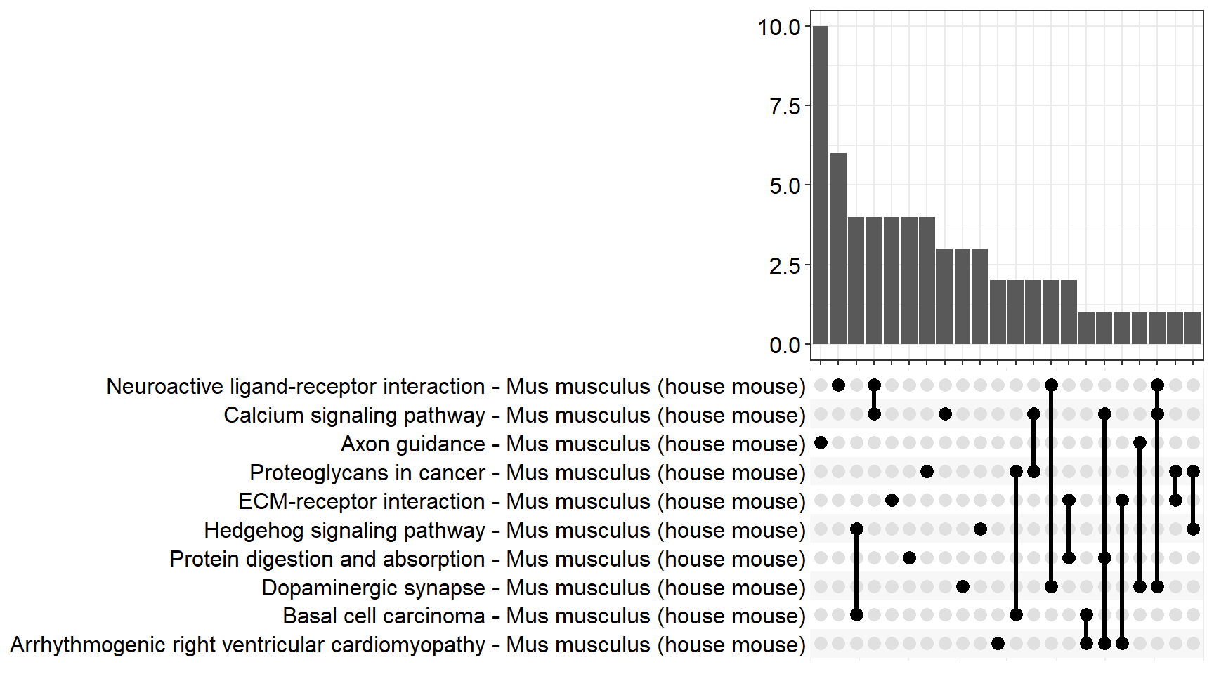
KEGG enrichment analysis is performed with the significant DE genes that have absolute FC > 1.5 ( genes from Limma). Top 30 most significant KEGG are displayed. All enriched KEGG pathways are exported.
KEGG pathway images reproduced by permission from Kanehisa Laboratories, September 2023
# chosing the pathways of interest
kegg_id <- c("mmu04670", "mmu04640", "mmu04270", "mmu04151", "mmu04510", "mmu04060")
kegg_pathway <- KEGGREST::keggGet(kegg_id)
enrichKEGG <- list()
enrichKEGG_all <- list()
enrichKEGG_sig <- list()
for (i in 1:length(fc)) {
x <- fc[i] %>% as.character()
# find enriched KEGG pathways
enrichKEGG[[x]] <- clusterProfiler::enrichKEGG(
gene = lmTreat_sig[[x]]$entrezid,
keyType = "kegg",
organism = "mmu",
pvalueCutoff = 0.05,
pAdjustMethod = "none"
)
enrichKEGG[[x]] <- enrichKEGG[[x]] %>%
clusterProfiler::setReadable(OrgDb = org.Mm.eg.db, keyType = "ENTREZID")
enrichKEGG_all[[x]] <- enrichKEGG[[x]]@result
# filter the significant and print top 30
enrichKEGG_sig[[x]] <- enrichKEGG_all[[x]] %>%
dplyr::filter(pvalue <= 0.05) %>%
separate(col = BgRatio, sep = "/", into = c("Total", "Universe")) %>%
dplyr::mutate(
logPval = -log(pvalue, 10),
GeneRatio = Count / as.numeric(Total)
) %>%
dplyr::select(c("Description", "GeneRatio", "pvalue", "logPval", "p.adjust", "qvalue", "geneID", "Count"))
# # at the beginnning of a word (after 35 characters), add a newline. shorten the y axis for dot plot
# enrichKEGG_sig[[x]]$Description <- sub(pattern = "(.{1,35})(?:$| )",
# replacement = "\\1\n",
# x = enrichKEGG_sig[[x]]$Description)
#
# # remove the additional newline at the end of the string
# enrichKEGG_sig[[x]]$Description <- sub(pattern = "\n$",
# replacement = "",
# x = enrichKEGG_sig[[x]]$Description)
}FC=1.05
p=1Table
enrichKEGG_sig[[p]] %>%
  dplyr::mutate_if(is.numeric, funs(as.character(signif(.,3)))) %>%
  DT(.,caption = "Significantly enriched KEGG pathways")
# kable(caption = "Significantly enriched KEGG pathways") %>%
# kable_styling(bootstrap_options = c("striped", "hover")) %>%
# scroll_box(height = "600px")Dot plot
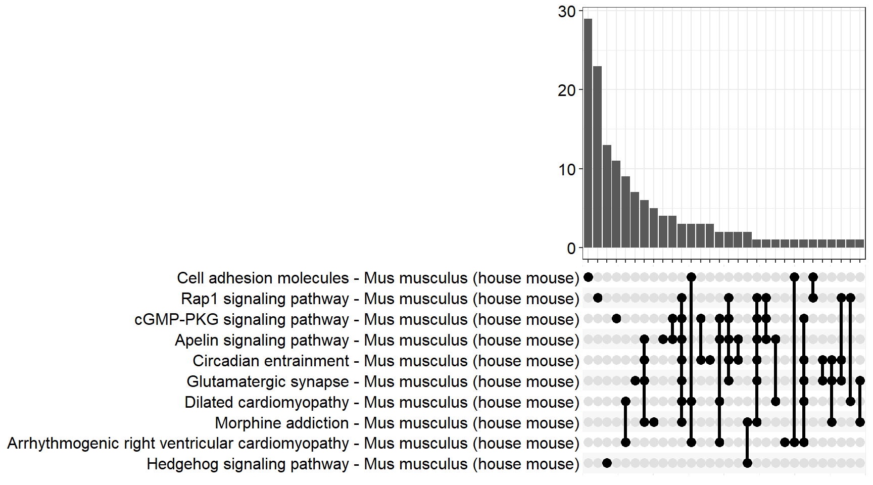
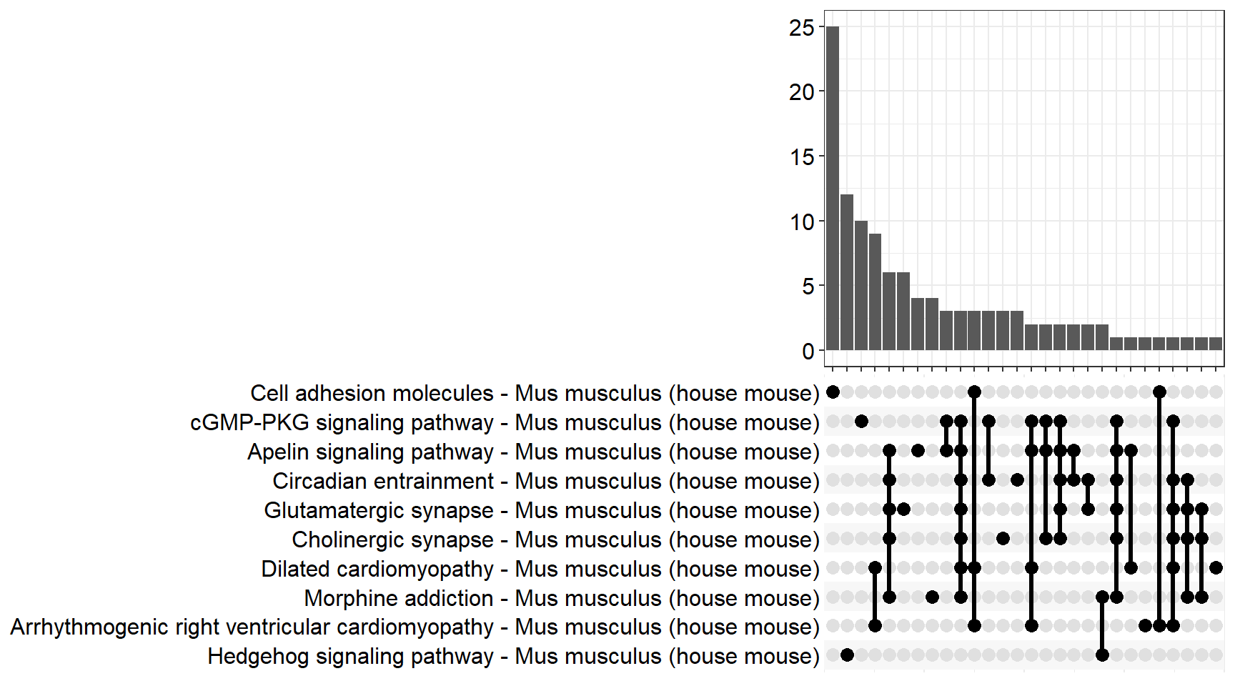
kegg_dot <- list()
upset=list()
for (i in 1:length(fc)) {
  x <- fc[i] %>% as.character()

  # dot plot, save
  kegg_dot[[x]] <- ggplot(enrichKEGG_sig[[x]][1:15, ]) +
    geom_point(aes(x = GeneRatio, y = reorder(Description, GeneRatio), colour = logPval, size = Count)) +
    scale_color_gradient(low = "dodgerblue3", high = "firebrick3", limits = c(0, NA)) +
    scale_size(range = c(1.5,5)) +
    ggtitle("KEGG Pathways") +
    ylab(label = "") +
    xlab(label = "Gene Ratio") +
    labs(color = expression("-log"[10] * "Pvalue"), size = "Gene Counts")
  ggsave(filename = paste0("kegg_dot_", fc[i], ".svg"), plot = kegg_dot[[x]] + pub, path = here::here("2_plots/kegg/"),
         width = 250, height = 130, units = "mm")

  upset[[x]] <- upsetplot(x = enrichKEGG[[x]], 10)
  ggsave(filename = paste0("upset_kegg_", fc[i], ".svg"), plot = upset[[x]], path = here::here("2_plots/kegg/"),
         width = 170, height = 130, units = "mm")
}

kegg_dot[[p]]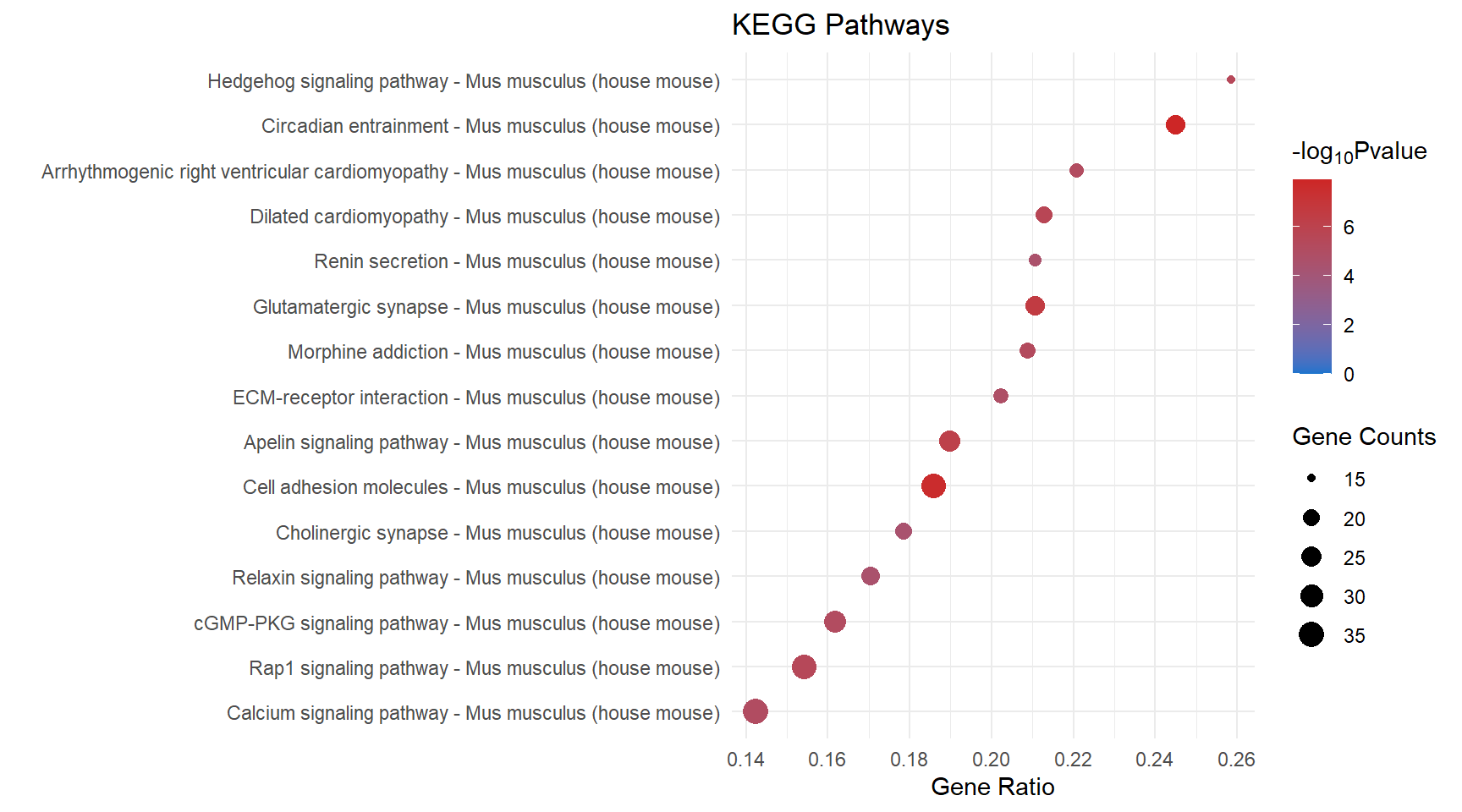
FC=1.1
p=p+1Table
enrichKEGG_sig[[p]] %>%
  dplyr::mutate_if(is.numeric, funs(as.character(signif(.,3)))) %>%
  DT(.,caption = "Significantly enriched KEGG pathways")
# kable(caption = "Significantly enriched KEGG pathways") %>%
# kable_styling(bootstrap_options = c("striped", "hover")) %>%
# scroll_box(height = "600px")Dot plot
kegg_dot[[p]]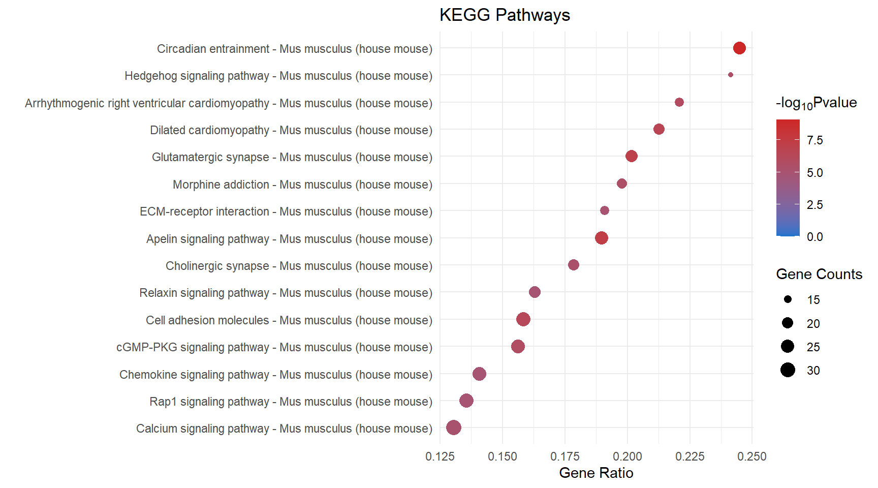
FC=1.5
p=p+1Table
enrichKEGG_sig[[p]] %>%
  dplyr::mutate_if(is.numeric, funs(as.character(signif(.,3)))) %>%
  DT(.,caption = "Significantly enriched KEGG pathways")
# kable(caption = "Significantly enriched KEGG pathways") %>%
# kable_styling(bootstrap_options = c("striped", "hover")) %>%
# scroll_box(height = "600px")Dot plot
kegg_dot[[p]]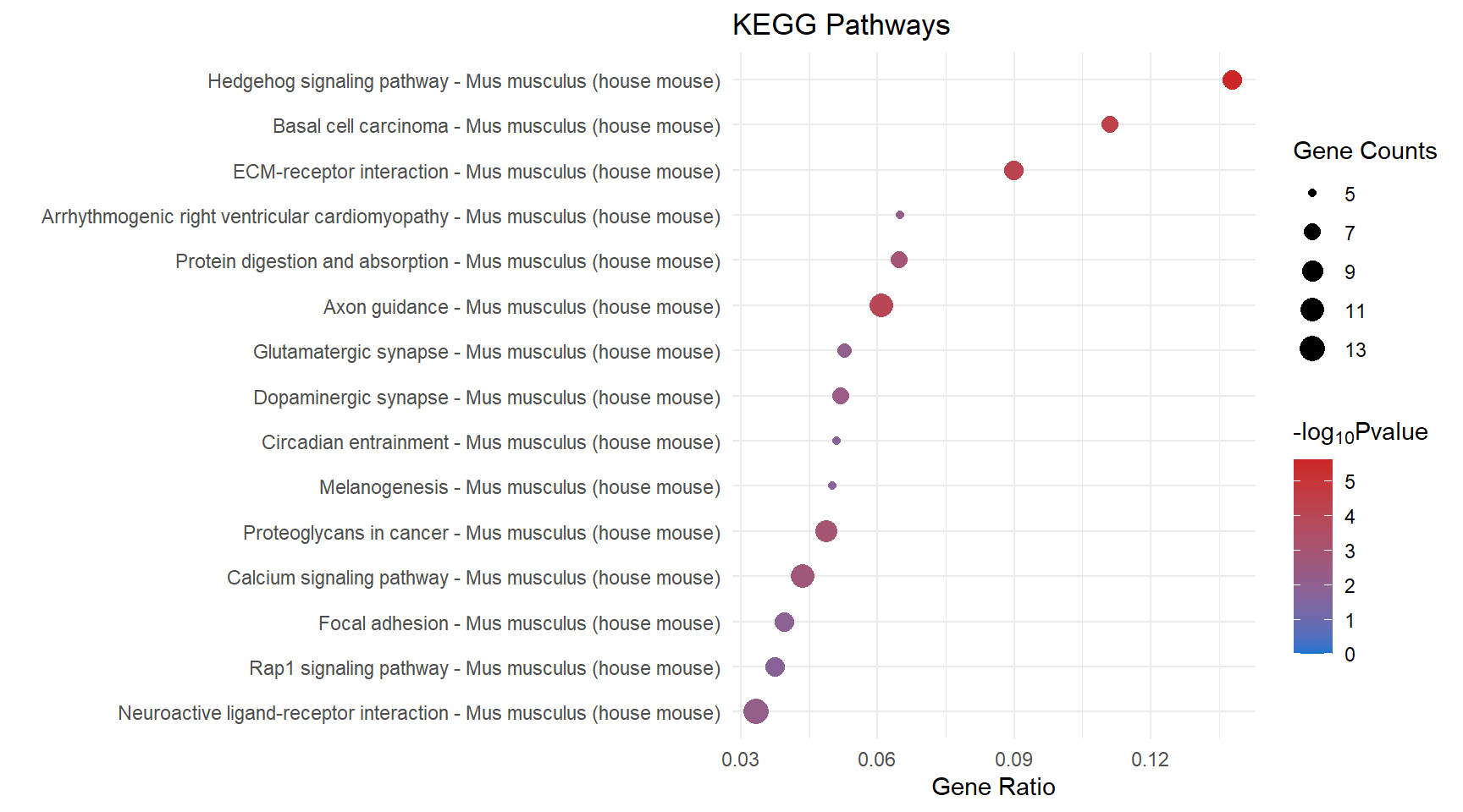
Pathway specific heatmaps
FC=1.05
p=1Leukocyte transendothelial migration
q=1Heatmap
# create df with normalised read counts with an additional entrezid column for binding
logCPM <- cpm(dge, prior.count = 3, log = TRUE)
logCPM <- logCPM[,1:7]
logCPM <- cbind(logCPM, dge$genes$entrezid)
rownames(logCPM) <- dge$genes$gene_name
colnames(logCPM) <- c("Control 1", "Control 2", "Control 4", "Intact 1", "Intact 2", "Intact 3", "Intact 4", "entrezid")

### full pathway method
# complete_pathway <- kegg_pathway[[1]]$GENE %>% as.data.frame()
# complete_pathway <- focal_adhesion[seq(1, nrow(focal_adhesion), 2),]
# match_complete_pathway <- logCPM[,"entrezid"] %in% complete_pathway


# df for heatmap annotation of sample group
anno <- as.factor(dge$samples$group) %>% as.data.frame()
anno <- anno[1:7,] %>% as.data.frame()
colnames(anno) <- "Sample Groups"
anno$`Sample Groups` <- gsub("CONT", "Control", anno$`Sample Groups`)
anno$`Sample Groups` <- gsub("INT", "Intact", anno$`Sample Groups`)
rownames(anno) <- colnames(logCPM[, 1:7])

# setting colour of sample group annotation

# original sample colours
# anno_colours <- c("#66C2A5", "#FC8D62")

# new sample colours
anno_colours <- c("#f8766d", "#a3a500")

names(anno_colours) <- c("Control", "Intact")
matrix <- list()
display_matrix <- list()
kegg_heat=list()
my_palette <- colorRampPalette(c(
rgb(32,121,226, maxColorValue = 255),
# rgb(144,203,180, maxColorValue = 255),
rgb(254,248,239, maxColorValue = 255),
# rgb(251,192,52, maxColorValue = 255),
rgb(226,46,45, maxColorValue = 255)))(n = 201)
for (i in 1:length(fc)) {
x <- fc[i] %>% as.character()
for (j in 1:length(kegg_id)) {
y <- kegg_pathway[[j]]$PATHWAY_MAP
partial <- enrichKEGG_all[[x]][, c("ID", "geneID")]
partial <- partial[kegg_id[j], "geneID"] %>% as.data.frame()
partial <- separate_rows(partial, ., sep = "/")
colnames(partial) <- "entrezid"
# heatmap matrix
match <- rownames(logCPM) %in% partial$entrezid
matrix[[x]][[y]] <- logCPM[match, c("Control 1", "Control 2", "Control 4", "Intact 1", "Intact 2", "Intact 3", "Intact 4")] %>% as.data.frame()
# changing the colname to numeric for some reason, cant remember
matrix[[x]][[y]][, c("Control 1", "Control 2", "Control 4", "Intact 1", "Intact 2", "Intact 3", "Intact 4")] <- as.numeric(as.character(unlist(matrix[[x]][[y]][, c("Control 1", "Control 2", "Control 4", "Intact 1", "Intact 2", "Intact 3", "Intact 4")])))
# display matrix
match2 <- lmTreat_sig[[x]][, "gene_name"] %in% partial$entrezid
display_matrix[[x]][[y]] <- lmTreat_sig[[x]][match2, c("gene_name", "logFC", "P.Value", "adj.P.Val", "description")] %>%
as.data.frame()
colnames(display_matrix[[x]][[y]]) <- c("Gene Name", "logFC", "P Value", "Adjusted P Value", "Description")
## Heatmap
kegg_heat[[x]][[y]] <- pheatmap(
mat = matrix[[x]][[y]],
### Publish
show_colnames = T,
main = paste0(y, "\n"),
legend = F,
annotation_legend = F,
fontsize = 10,
fontsize_col = 11,
fontsize_number = 7,
fontsize_row = 10,
treeheight_row = 25,
treeheight_col = 10,
cluster_cols = T,
clustering_distance_rows = "euclidean",
legend_breaks = c(seq(-3, 11, by = .5), 1.4),
legend_labels = c(seq(-3, 11, by = .5), "Z-Score"),
angle_col = 90,
cutree_cols = 2,
cutree_rows = 2,
color = my_palette,
scale = "row",
border_color = NA,
annotation_col = anno,
annotation_colors = list("Sample Groups" = anno_colours),
annotation_names_col = F,
annotation = T,
silent = T,
labels_row = as.expression(lapply(rownames(matrix[[x]][[y]]), function(a) bquote(italic(.(a)))))
) %>% as.ggplot()
# save
ggsave(filename = paste0("heat_", x, "_", y, ".svg"),
plot = kegg_heat[[x]][[y]],
path = here::here("2_plots/kegg/"),
width = 166,
height = 250,
units = "mm")}
}kegg_heat[[p]][[q]]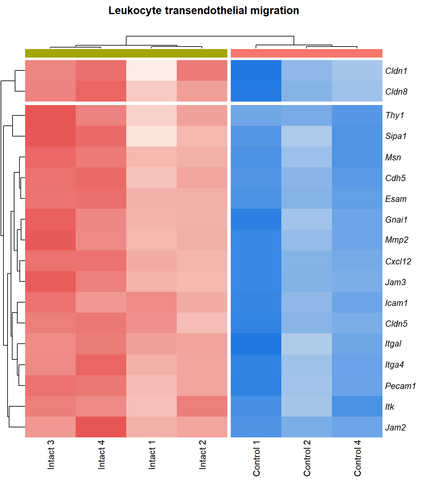
Table
display_matrix[[p]][[q]] %>%
  dplyr::mutate_if(is.numeric, funs(as.character(signif(.,3)))) %>%
  DT(.,caption = "DE genes")
# kable() %>%
# kable_styling(bootstrap_options = c("striped", "hover")) %>%
# scroll_box(height = "600px")Pathview
# adjusting the kegg id to suit the parameters of the pathview funtion
adj.keggID <- gsub("mmu", "", kegg_id)

for (i in 1:length(fc)) {
  x <- fc[i] %>% as.character()

  # extract the logFC from the DE gene list
  pathview_table <- dplyr::select(.data = lmTreat_sig[[x]], c("logFC")) %>% as.matrix()

  # run pathview with Ensembl ID instead of entrezID
  pathview <- pathview(
    gene.data = pathview_table[, 1],
    gene.idtype = "ENSEMBL",
    pathway.id = adj.keggID,
    species = "mmu",
    out.suffix = "pv",
    kegg.dir = here::here("2_plots/kegg/"),
    kegg.native = T
  )

  # move the result file to the plot directory
  file.rename(
    from = paste0("mmu", adj.keggID, ".pv.png"),
    to = here::here(paste0("docs/figure/kegg.Rmd/pv_", x, "_", kegg_id, ".png"))
  )
}
[1] "Note: 163 of 1629 unique input IDs unmapped."[1] "Note: 148 of 1447 unique input IDs unmapped."[1] "Note: 60 of 388 unique input IDs unmapped."
Hematopoietic cell lineage
q=q+1Heatmap
kegg_heat[[p]][[q]]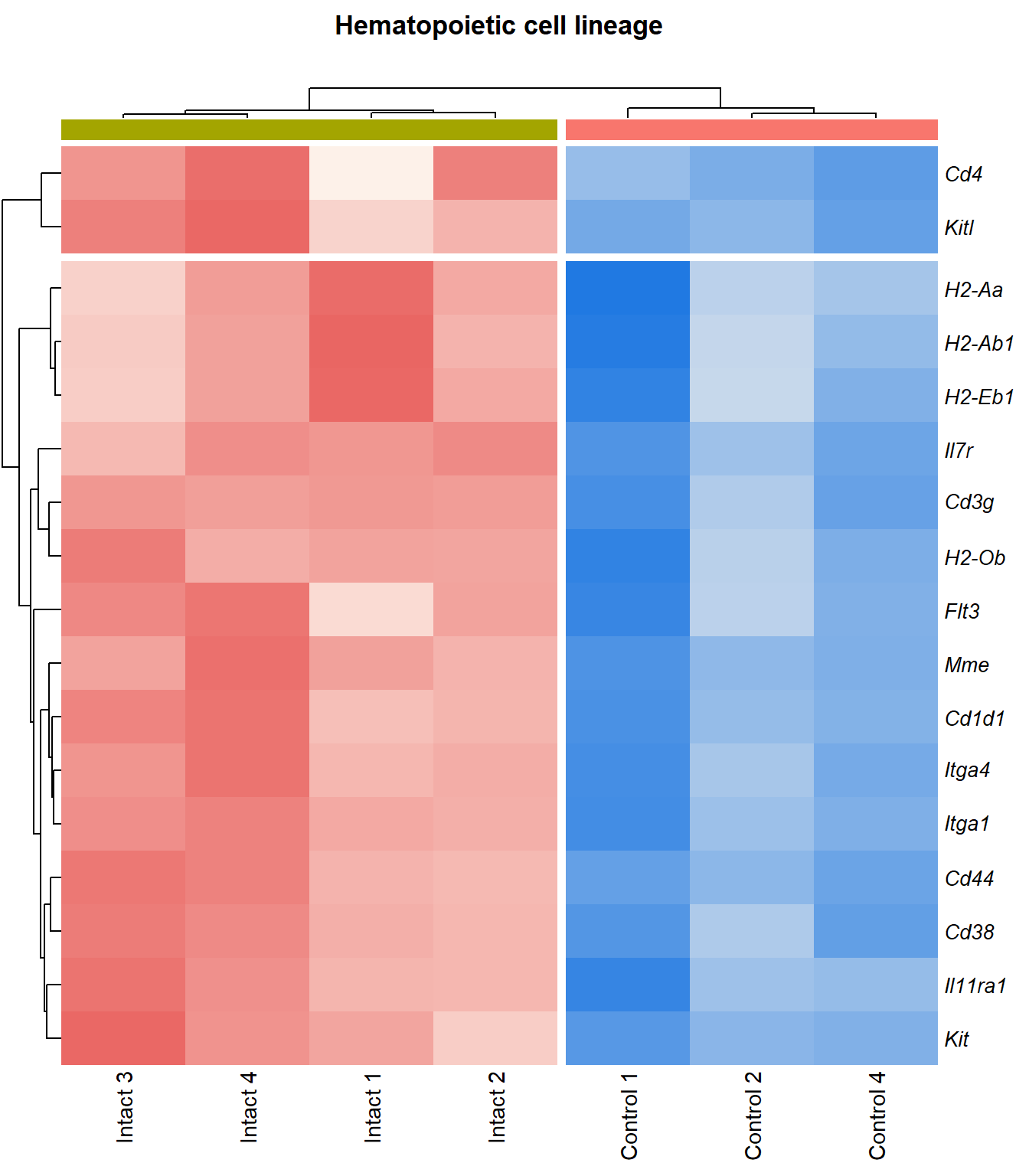
Tables
display_matrix[[p]][[q]] %>%
  dplyr::mutate_if(is.numeric, funs(as.character(signif(.,3)))) %>%
  DT(.,caption = "DE genes")
# kable() %>%
# kable_styling(bootstrap_options = c("striped", "hover")) %>%
# scroll_box(height = "600px")Pathview

Vascular smooth muscle contraction
q=q+1Heatmap
kegg_heat[[p]][[q]]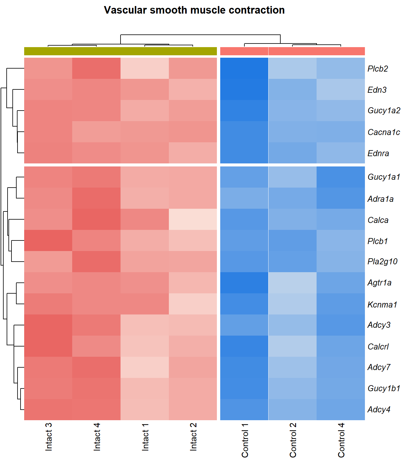
Tables
display_matrix[[p]][[q]] %>%
  dplyr::mutate_if(is.numeric, funs(as.character(signif(.,3)))) %>%
  DT(.,caption = "DE genes")
# kable() %>%
# kable_styling(bootstrap_options = c("striped", "hover")) %>%
# scroll_box(height = "600px")Pathview

PI3K-Akt signaling pathway
q=q+1Heatmap
kegg_heat[[p]][[q]]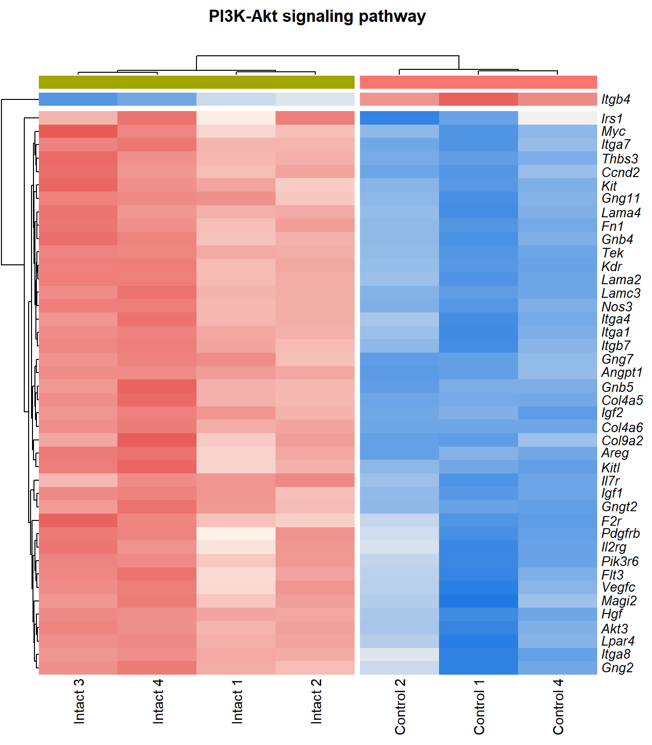
Tables
display_matrix[[p]][[q]] %>%
  dplyr::mutate_if(is.numeric, funs(as.character(signif(.,3)))) %>%
  DT(.,caption = "DE genes")
# kable() %>%
# kable_styling(bootstrap_options = c("striped", "hover")) %>%
# scroll_box(height = "600px")Pathview

Focal adhesion
q=q+1Heatmap
kegg_heat[[p]][[q]]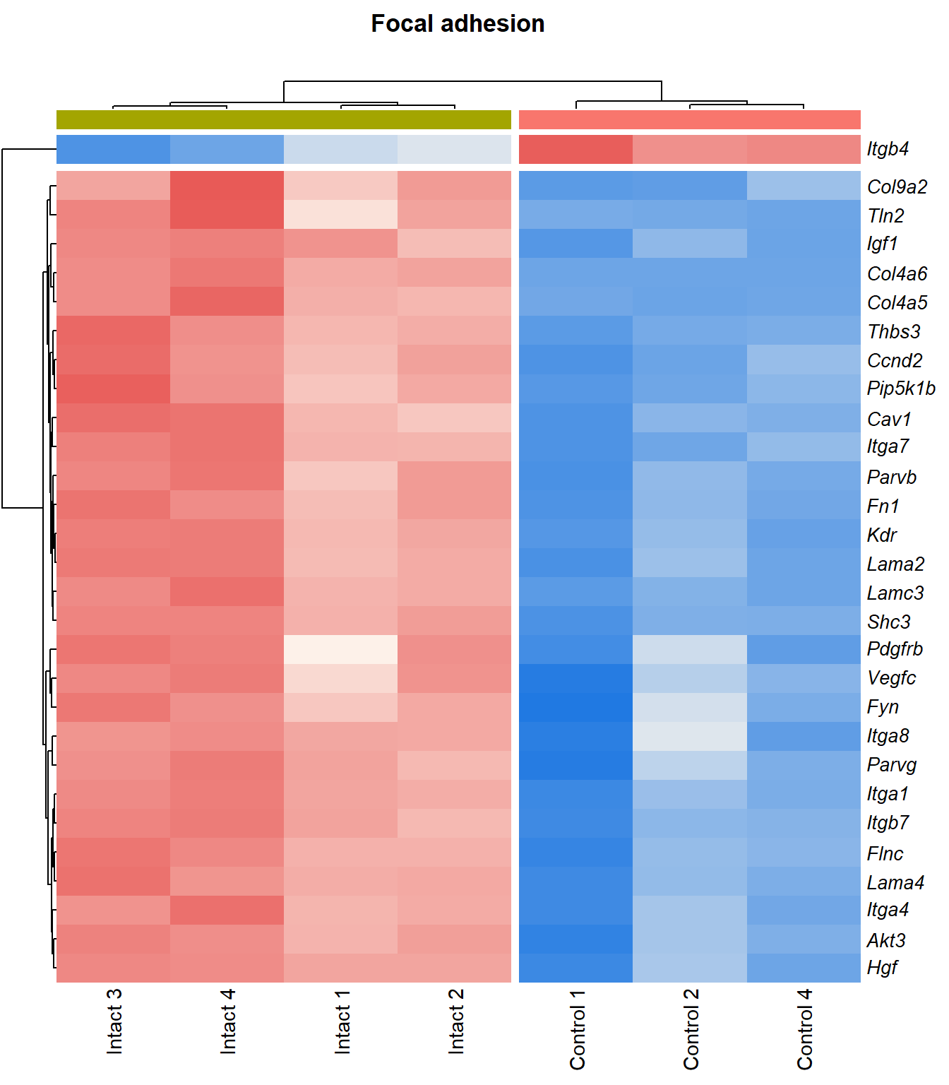
Tables
display_matrix[[p]][[q]] %>%
  dplyr::mutate_if(is.numeric, funs(as.character(signif(.,3)))) %>%
  DT(.,caption = "DE genes")
# kable() %>%
# kable_styling(bootstrap_options = c("striped", "hover")) %>%
# scroll_box(height = "600px")Pathview

Cytokine-cytokine receptor interaction
q=q+1Heatmap
kegg_heat[[p]][[q]]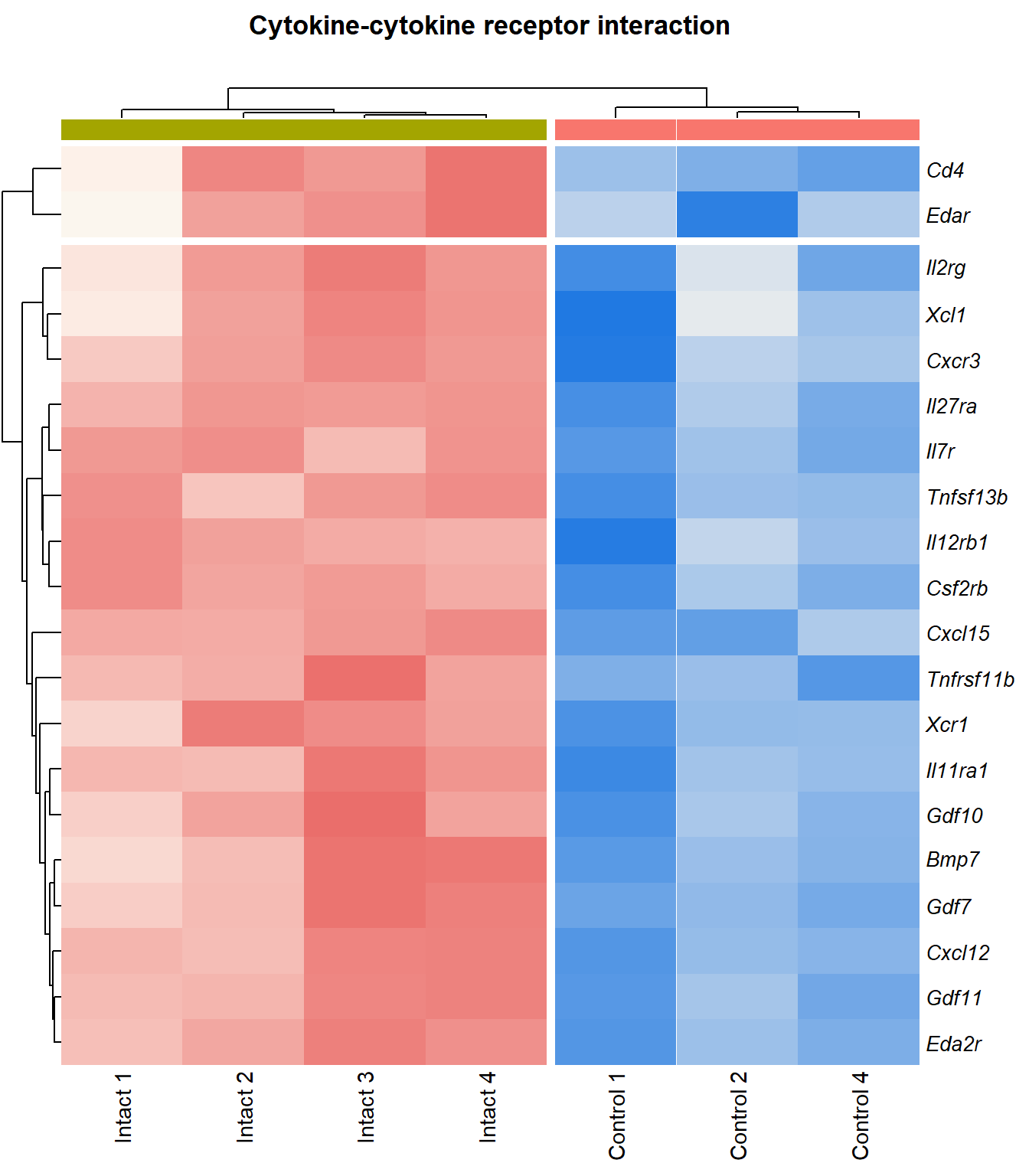
Tables
display_matrix[[p]][[q]] %>%
  dplyr::mutate_if(is.numeric, funs(as.character(signif(.,3)))) %>%
  DT(.,caption = "DE genes")
# kable() %>%
# kable_styling(bootstrap_options = c("striped", "hover")) %>%
# scroll_box(height = "600px")Pathview

FC=1.1
p=p+1Leukocyte transendothelial migration
q=1Heatmap
kegg_heat[[p]][[q]]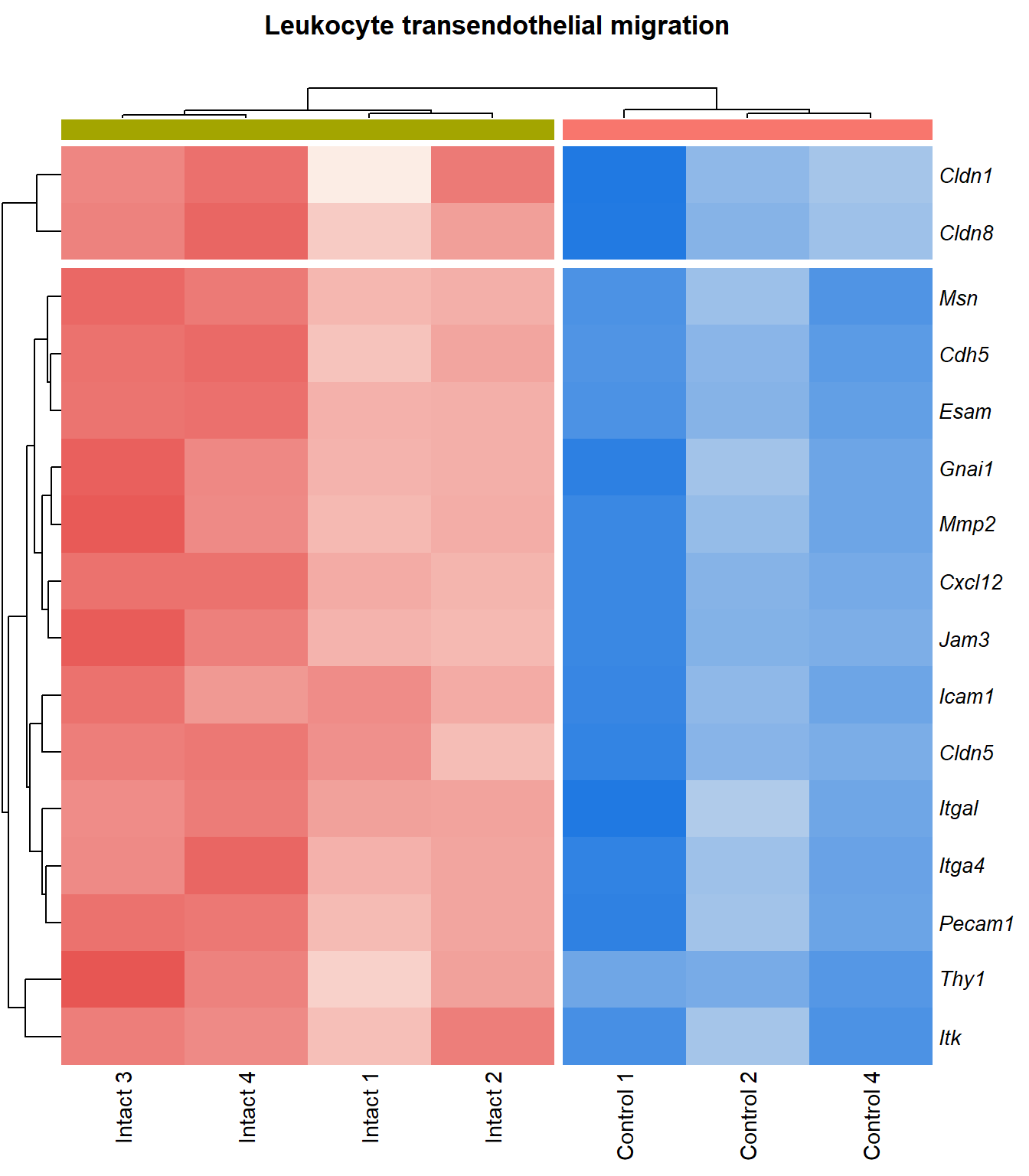
Tables
display_matrix[[p]][[q]] %>%
  dplyr::mutate_if(is.numeric, funs(as.character(signif(.,3)))) %>%
  DT(.,caption = "DE genes")
# kable() %>%
# kable_styling(bootstrap_options = c("striped", "hover")) %>%
# scroll_box(height = "600px")Pathview

Hematopoietic cell lineage
q=q+1Heatmap
kegg_heat[[p]][[q]]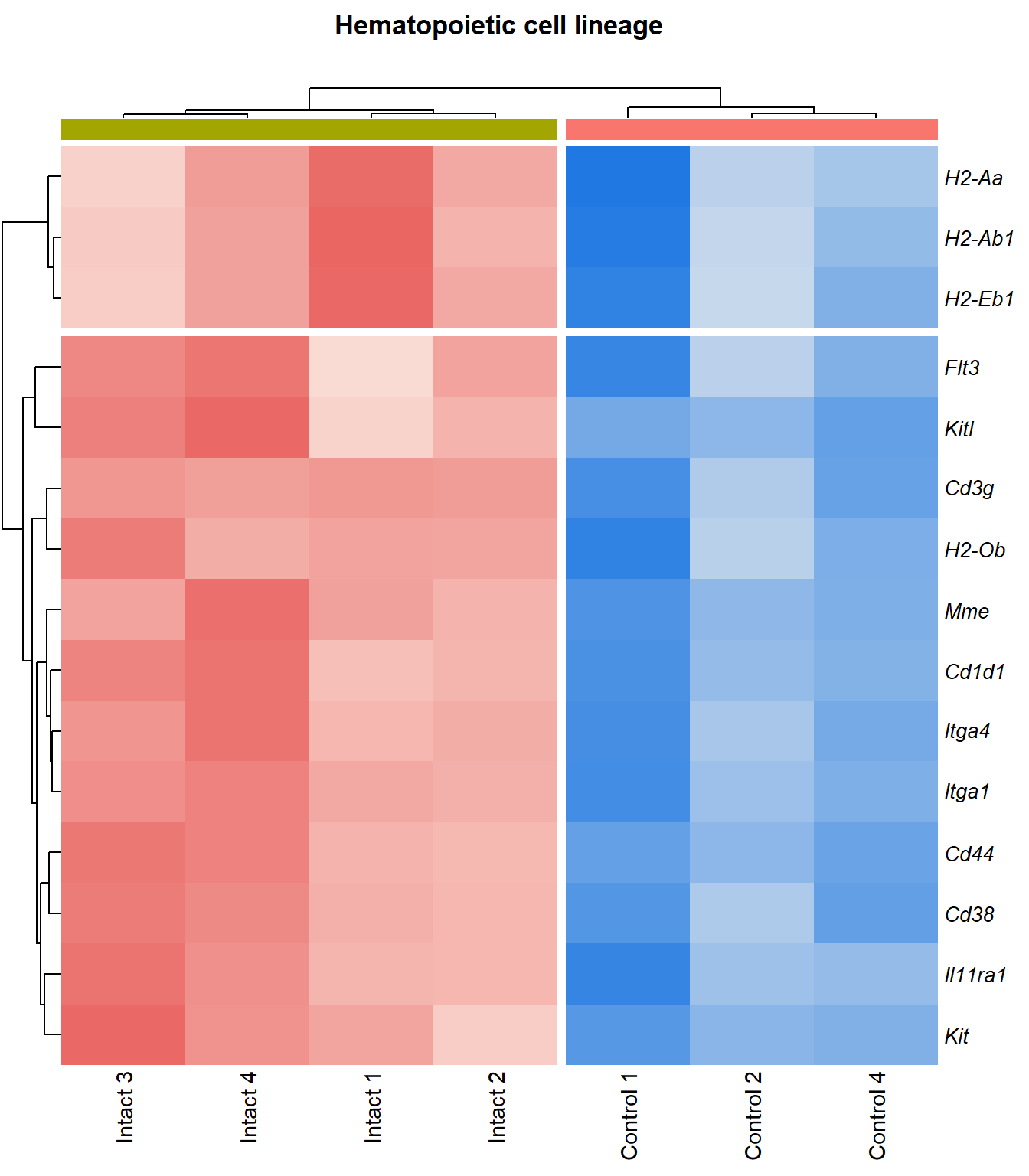
Tables
display_matrix[[p]][[q]] %>%
  dplyr::mutate_if(is.numeric, funs(as.character(signif(.,3)))) %>%
  DT(.,caption = "DE genes")
# kable() %>%
# kable_styling(bootstrap_options = c("striped", "hover")) %>%
# scroll_box(height = "600px")Pathview

Vascular smooth muscle contraction
q=q+1Heatmap
kegg_heat[[p]][[q]]
Tables
display_matrix[[p]][[q]] %>%
  dplyr::mutate_if(is.numeric, funs(as.character(signif(.,3)))) %>%
  DT(.,caption = "DE genes")
# kable() %>%
# kable_styling(bootstrap_options = c("striped", "hover")) %>%
# scroll_box(height = "600px")Pathview

PI3K-Akt signaling pathway
q=q+1Heatmap
kegg_heat[[p]][[q]]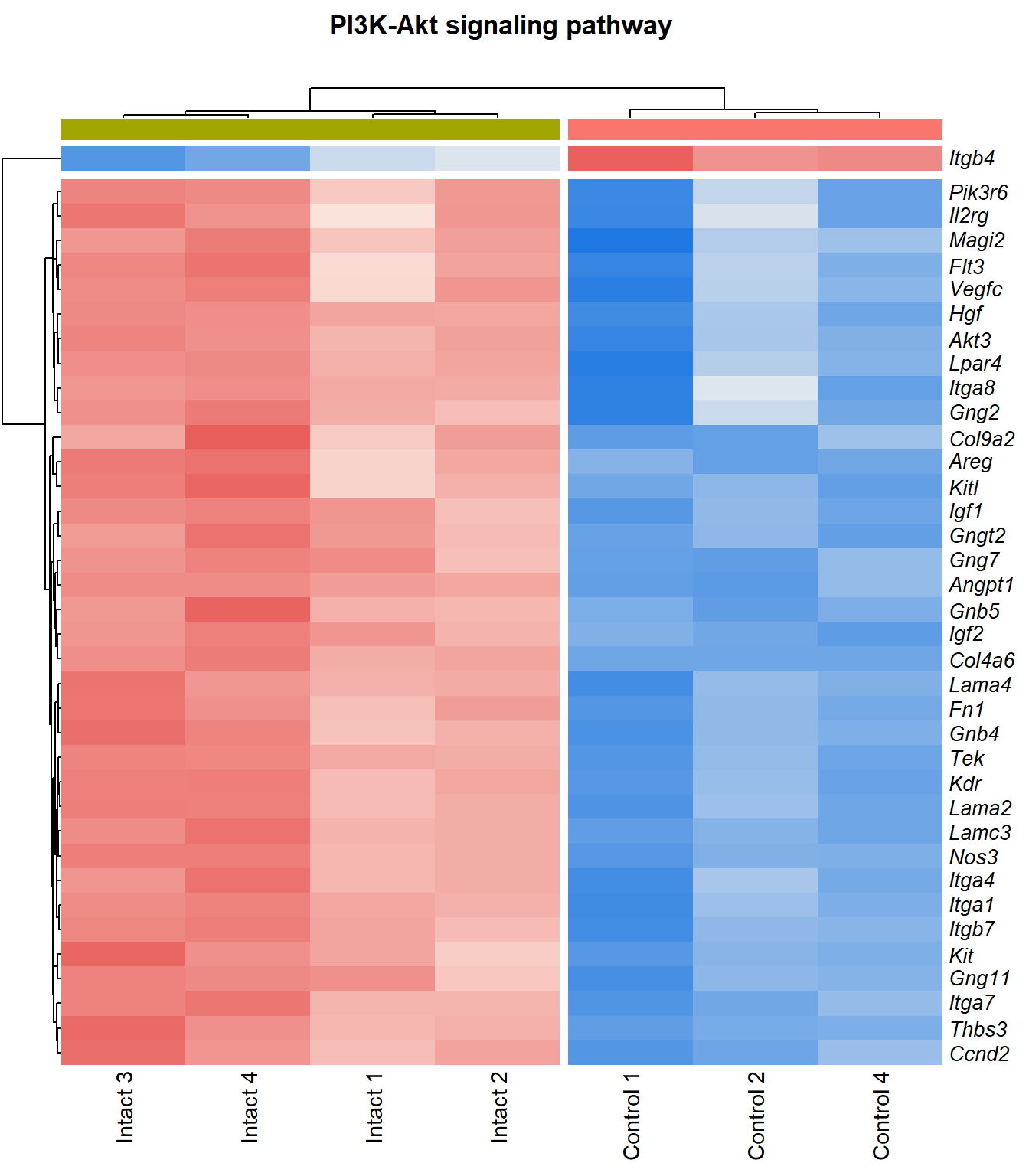
Tables
display_matrix[[p]][[q]] %>%
  dplyr::mutate_if(is.numeric, funs(as.character(signif(.,3)))) %>%
  DT(.,caption = "DE genes")
# kable() %>%
# kable_styling(bootstrap_options = c("striped", "hover")) %>%
# scroll_box(height = "600px")Pathview

Focal adhesion
q=q+1Heatmap
kegg_heat[[p]][[q]]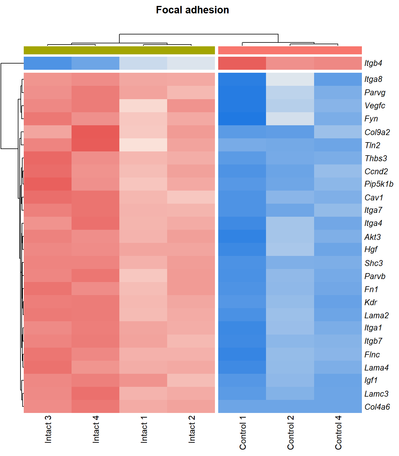
Tables
display_matrix[[p]][[q]] %>%
  dplyr::mutate_if(is.numeric, funs(as.character(signif(.,3)))) %>%
  DT(.,caption = "DE genes")
# kable() %>%
# kable_styling(bootstrap_options = c("striped", "hover")) %>%
# scroll_box(height = "600px")Pathview

Cytokine-cytokine receptor interaction
q=q+1Heatmap
kegg_heat[[p]][[q]]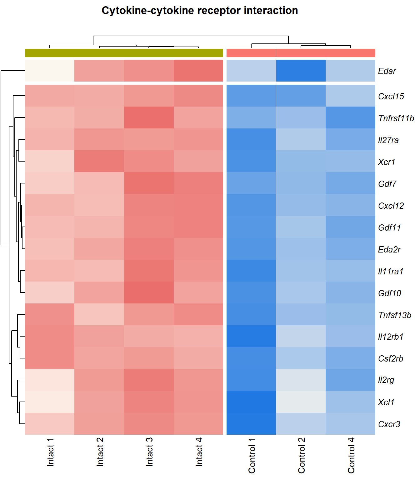
Tables
display_matrix[[p]][[q]] %>%
  dplyr::mutate_if(is.numeric, funs(as.character(signif(.,3)))) %>%
  DT(.,caption = "DE genes")
# kable() %>%
# kable_styling(bootstrap_options = c("striped", "hover")) %>%
# scroll_box(height = "600px")Pathview

FC=1.5
p=p+1Leukocyte transendothelial migration
q=1Heatmap
kegg_heat[[p]][[q]]
Tables
display_matrix[[p]][[q]] %>%
  dplyr::mutate_if(is.numeric, funs(as.character(signif(.,3)))) %>%
  DT(.,caption = "DE genes")
# kable() %>%
# kable_styling(bootstrap_options = c("striped", "hover")) %>%
# scroll_box(height = "600px")Pathview
Hematopoietic cell lineage
q=q+1Heatmap
kegg_heat[[p]][[q]]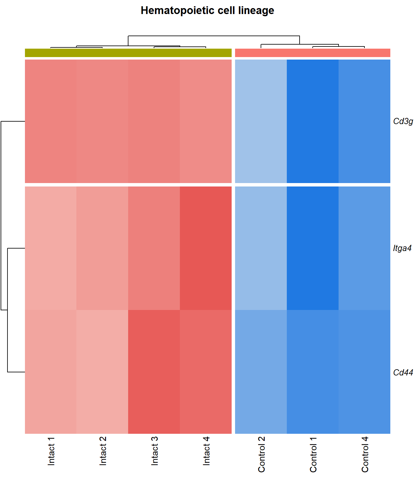
Tables
display_matrix[[p]][[q]] %>%
  dplyr::mutate_if(is.numeric, funs(as.character(signif(.,3)))) %>%
  DT(.,caption = "DE genes")
# kable() %>%
# kable_styling(bootstrap_options = c("striped", "hover")) %>%
# scroll_box(height = "600px")Pathview
Vascular smooth muscle contraction
q=q+1Heatmap
kegg_heat[[p]][[q]]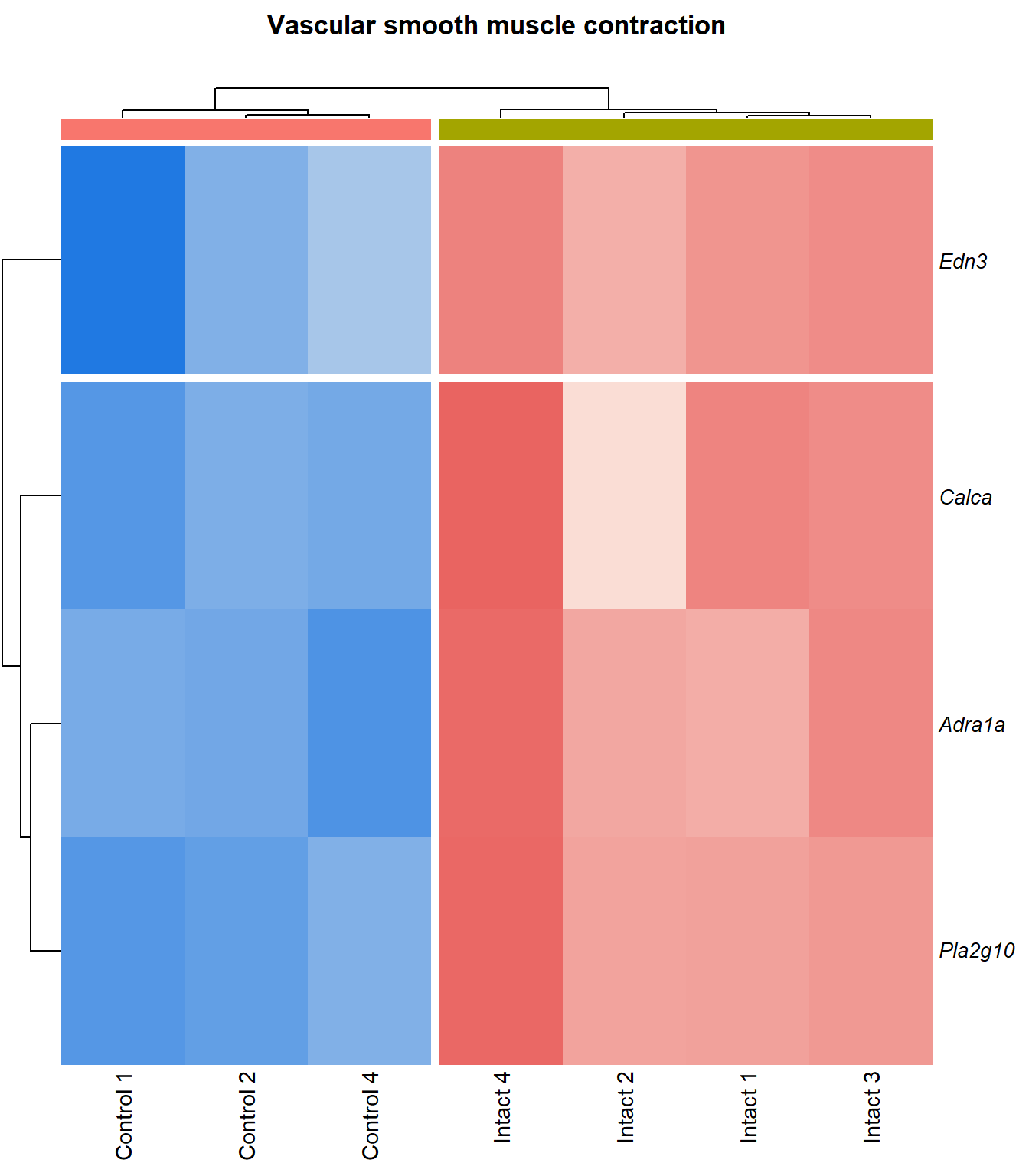
Tables
display_matrix[[p]][[q]] %>%
  dplyr::mutate_if(is.numeric, funs(as.character(signif(.,3)))) %>%
  DT(.,caption = "DE genes")
# kable() %>%
# kable_styling(bootstrap_options = c("striped", "hover")) %>%
# scroll_box(height = "600px")Pathview
PI3K-Akt signaling pathway
q=q+1Heatmap
kegg_heat[[p]][[q]]
Tables
display_matrix[[p]][[q]] %>%
  dplyr::mutate_if(is.numeric, funs(as.character(signif(.,3)))) %>%
  DT(.,caption = "DE genes")
# kable() %>%
# kable_styling(bootstrap_options = c("striped", "hover")) %>%
# scroll_box(height = "600px")Pathview
Focal adhesion
q=q+1Heatmap
kegg_heat[[p]][[q]]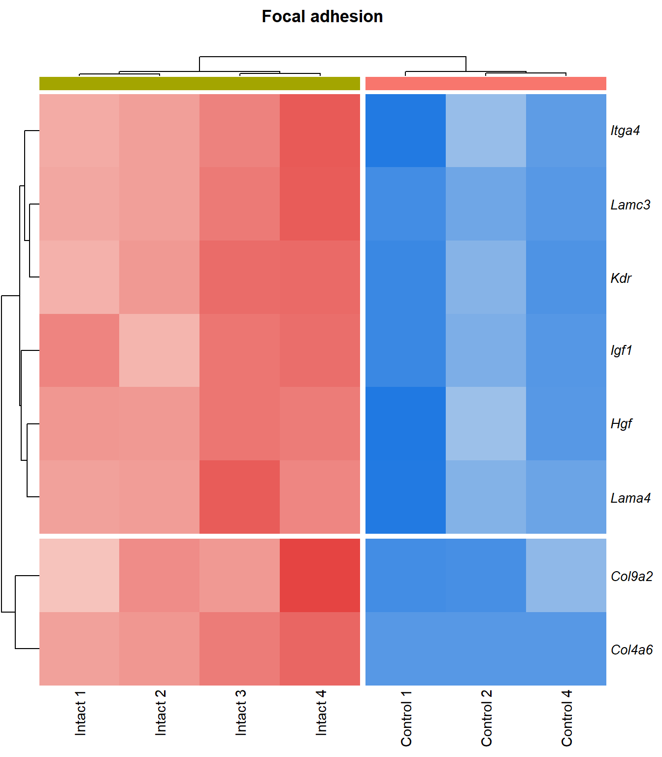
Tables
display_matrix[[p]][[q]] %>%
  dplyr::mutate_if(is.numeric, funs(as.character(signif(.,3)))) %>%
  DT(.,caption = "DE genes")
# kable() %>%
# kable_styling(bootstrap_options = c("striped", "hover")) %>%
# scroll_box(height = "600px")Pathview
Cytokine-cytokine receptor interaction
q=q+1Heatmap
kegg_heat[[p]][[q]]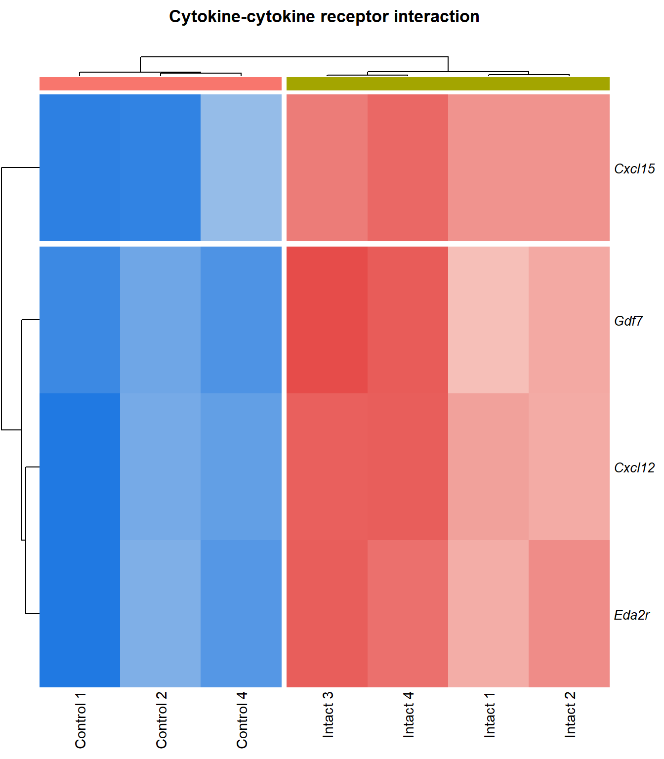
Tables
display_matrix[[p]][[q]] %>%
  dplyr::mutate_if(is.numeric, funs(as.character(signif(.,3)))) %>%
  DT(.,caption = "DE genes")
# kable() %>%
# kable_styling(bootstrap_options = c("striped", "hover")) %>%
# scroll_box(height = "600px")Pathview
Export Data
# save to csv
writexl::write_xlsx(x = enrichKEGG_all, here::here("3_output/enrichKEGG_all.xlsx"))
writexl::write_xlsx(x = enrichKEGG_sig, here::here("3_output/enrichKEGG_sig.xlsx"))
sessionInfo()R version 4.3.1 (2023-06-16 ucrt)
Platform: x86_64-w64-mingw32/x64 (64-bit)
Running under: Windows 10 x64 (build 19045)
Matrix products: default
locale:
[1] LC_COLLATE=English_Australia.utf8 LC_CTYPE=English_Australia.utf8
[3] LC_MONETARY=English_Australia.utf8 LC_NUMERIC=C
[5] LC_TIME=English_Australia.utf8
time zone: Australia/Adelaide
tzcode source: internal
attached base packages:
[1] stats4 grid stats graphics grDevices utils datasets
[8] methods base
other attached packages:
[1] pathview_1.40.0 enrichplot_1.20.1 org.Mm.eg.db_3.17.0
[4] AnnotationDbi_1.62.2 IRanges_2.34.1 S4Vectors_0.38.1
[7] Biobase_2.60.0 BiocGenerics_0.46.0 clusterProfiler_4.8.3
[10] Glimma_2.10.0 edgeR_3.42.4 limma_3.56.2
[13] ggrepel_0.9.3 ggbiplot_0.55 scales_1.2.1
[16] plyr_1.8.8 ggpubr_0.6.0 ggplotify_0.1.2
[19] DT_0.29 pheatmap_1.0.12 cowplot_1.1.1
[22] viridis_0.6.4 viridisLite_0.4.2 pander_0.6.5
[25] kableExtra_1.3.4 KEGGREST_1.40.0 lubridate_1.9.2
[28] forcats_1.0.0 stringr_1.5.0 purrr_1.0.1
[31] tidyr_1.3.0 ggplot2_3.4.3 tidyverse_2.0.0
[34] reshape2_1.4.4 tibble_3.2.1 readr_2.1.4
[37] magrittr_2.0.3 dplyr_1.1.2
loaded via a namespace (and not attached):
[1] splines_4.3.1 later_1.3.1
[3] bitops_1.0-7 polyclip_1.10-4
[5] graph_1.78.0 XML_3.99-0.14
[7] lifecycle_1.0.3 rstatix_0.7.2
[9] rprojroot_2.0.3 lattice_0.21-8
[11] MASS_7.3-60 crosstalk_1.2.0
[13] backports_1.4.1 sass_0.4.7
[15] rmarkdown_2.24 jquerylib_0.1.4
[17] yaml_2.3.7 httpuv_1.6.11
[19] DBI_1.1.3 RColorBrewer_1.1-3
[21] abind_1.4-5 zlibbioc_1.46.0
[23] rvest_1.0.3 GenomicRanges_1.52.0
[25] ggraph_2.1.0 RCurl_1.98-1.12
[27] yulab.utils_0.0.9 tweenr_2.0.2
[29] git2r_0.32.0 GenomeInfoDbData_1.2.10
[31] tidytree_0.4.5 svglite_2.1.1
[33] codetools_0.2-19 DelayedArray_0.26.7
[35] DOSE_3.26.1 xml2_1.3.5
[37] ggforce_0.4.1 tidyselect_1.2.0
[39] aplot_0.2.1 farver_2.1.1
[41] matrixStats_1.0.0 webshot_0.5.5
[43] jsonlite_1.8.7 ellipsis_0.3.2
[45] tidygraph_1.2.3 systemfonts_1.0.4
[47] tools_4.3.1 ragg_1.2.5
[49] treeio_1.24.3 Rcpp_1.0.11
[51] glue_1.6.2 gridExtra_2.3
[53] here_1.0.1 xfun_0.39
[55] DESeq2_1.40.2 qvalue_2.32.0
[57] MatrixGenerics_1.12.3 GenomeInfoDb_1.36.3
[59] withr_2.5.0 fastmap_1.1.1
[61] fansi_1.0.4 digest_0.6.33
[63] timechange_0.2.0 R6_2.5.1
[65] gridGraphics_0.5-1 textshaping_0.3.6
[67] colorspace_2.1-0 GO.db_3.17.0
[69] RSQLite_2.3.1 utf8_1.2.3
[71] generics_0.1.3 data.table_1.14.8
[73] graphlayouts_1.0.0 httr_1.4.7
[75] htmlwidgets_1.6.2 S4Arrays_1.0.6
[77] scatterpie_0.2.1 whisker_0.4.1
[79] pkgconfig_2.0.3 gtable_0.3.4
[81] blob_1.2.4 workflowr_1.7.1
[83] XVector_0.40.0 shadowtext_0.1.2
[85] htmltools_0.5.5 carData_3.0-5
[87] fgsea_1.26.0 ggupset_0.3.0
[89] png_0.1-8 ggfun_0.1.3
[91] knitr_1.44 rstudioapi_0.15.0
[93] tzdb_0.4.0 curl_5.0.2
[95] nlme_3.1-163 org.Hs.eg.db_3.17.0
[97] cachem_1.0.8 parallel_4.3.1
[99] HDO.db_0.99.1 pillar_1.9.0
[101] vctrs_0.6.3 promises_1.2.0.1
[103] car_3.1-2 Rgraphviz_2.44.0
[105] KEGGgraph_1.60.0 evaluate_0.21
[107] cli_3.6.1 locfit_1.5-9.8
[109] compiler_4.3.1 rlang_1.1.1
[111] crayon_1.5.2 ggsignif_0.6.4
[113] labeling_0.4.3 fs_1.6.3
[115] writexl_1.4.2 stringi_1.7.12
[117] BiocParallel_1.34.2 munsell_0.5.0
[119] Biostrings_2.68.1 lazyeval_0.2.2
[121] GOSemSim_2.26.1 Matrix_1.6-1
[123] hms_1.1.3 patchwork_1.1.3
[125] bit64_4.0.5 SummarizedExperiment_1.30.2
[127] igraph_1.5.1 broom_1.0.5
[129] memoise_2.0.1 bslib_0.5.1
[131] ggtree_3.8.2 fastmatch_1.1-4
[133] bit_4.0.5 downloader_0.4
[135] gson_0.1.0 ape_5.7-1