Last updated: 2023-09-16

Checks: 7 0

Knit directory: Mouse_endometrial_transcriptome_2023/1_analysis/

This reproducible R Markdown analysis was created with workflowr (version 1.7.1). The Checks tab describes the reproducibility checks that were applied when the results were created. The Past versions tab lists the development history.

R Markdown file: up-to-date

Great! Since the R Markdown file has been committed to the Git repository, you know the exact version of the code that produced these results.

Environment: empty

Great job! The global environment was empty. Objects defined in the global environment can affect the analysis in your R Markdown file in unknown ways. For reproduciblity it’s best to always run the code in an empty environment.

Seed: set.seed(12345)

The command set.seed(12345) was run prior to running the code in the R Markdown file. Setting a seed ensures that any results that rely on randomness, e.g. subsampling or permutations, are reproducible.

Session information: recorded

Great job! Recording the operating system, R version, and package versions is critical for reproducibility.

Cache: none

Nice! There were no cached chunks for this analysis, so you can be confident that you successfully produced the results during this run.

File paths: relative

Great job! Using relative paths to the files within your workflowr project makes it easier to run your code on other machines.

Repository version: 18c6463

Great! You are using Git for version control. Tracking code development and connecting the code version to the results is critical for reproducibility.

The results in this page were generated with repository version 18c6463. See the Past versions tab to see a history of the changes made to the R Markdown and HTML files.

Note that you need to be careful to ensure that all relevant files for the analysis have been committed to Git prior to generating the results (you can use wflow_publish or wflow_git_commit). workflowr only checks the R Markdown file, but you know if there are other scripts or data files that it depends on. Below is the status of the Git repository when the results were generated:


Ignored files:
    Ignored:    .Rproj.user/

Untracked files:
    Untracked:  .gitignore
    Untracked:  0_data/RDS_objects/DT.rds

Unstaged changes:
    Modified:   0_data/RDS_objects/dge.rds
    Modified:   0_data/RDS_objects/enrichGO.rds
    Modified:   0_data/RDS_objects/enrichGO_sig.rds
    Modified:   0_data/RDS_objects/fc.rds
    Modified:   0_data/RDS_objects/lfc.rds
    Modified:   0_data/RDS_objects/lmTreat.rds
    Modified:   0_data/RDS_objects/lmTreat_all.rds
    Modified:   0_data/RDS_objects/lmTreat_sig.rds
    Modified:   0_data/RDS_objects/pub.rds
    Deleted:    1_analysis/mmu04060.pv.png
    Deleted:    1_analysis/mmu04151.pv.png
    Deleted:    1_analysis/mmu04270.pv.png
    Deleted:    1_analysis/mmu04510.pv.png
    Deleted:    1_analysis/mmu04640.pv.png
    Deleted:    1_analysis/mmu04670.pv.png
    Modified:   2_plots/de/pval_1.05.svg
    Modified:   2_plots/de/pval_1.1.svg
    Modified:   2_plots/de/pval_1.5.svg
    Modified:   2_plots/go/bp_dot_1.05.svg
    Modified:   2_plots/go/bp_dot_1.5.svg
    Modified:   2_plots/go/cc_dot_1.05.svg
    Modified:   2_plots/go/cc_dot_1.5.svg
    Modified:   2_plots/go/mf_dot_1.5.svg
    Modified:   2_plots/go/upset_1.05.svg
    Modified:   2_plots/go/upset_1.1.svg
    Modified:   2_plots/go/upset_1.5.svg
    Modified:   2_plots/ipa/Cell-To-Cell Signaling.svg
    Modified:   2_plots/ipa/diseaseAndFunction.svg
    Modified:   2_plots/ipa/pathways.svg
    Modified:   2_plots/kegg/kegg_dot_1.05.svg
    Modified:   2_plots/kegg/kegg_dot_1.1.svg
    Modified:   2_plots/kegg/kegg_dot_1.5.svg
    Modified:   2_plots/kegg/upset_kegg_1.05.svg
    Modified:   2_plots/kegg/upset_kegg_1.1.svg
    Modified:   2_plots/kegg/upset_kegg_1.5.svg
    Modified:   2_plots/qc/PCA_IntvsCont.svg
    Modified:   2_plots/qc/counts_after_filtering_3_3.svg
    Modified:   2_plots/qc/counts_before_after_filtering_3_3.svg
    Modified:   2_plots/qc/counts_before_filtering.svg
    Modified:   2_plots/qc/library_size.svg
    Modified:   2_plots/reactome/react_dot_1.05.svg
    Modified:   2_plots/reactome/react_dot_1.1.svg
    Modified:   2_plots/reactome/react_dot_1.5.svg
    Modified:   2_plots/reactome/upset_react_1.05.svg
    Modified:   2_plots/reactome/upset_react_1.1.svg
    Modified:   2_plots/reactome/upset_react_1.5.svg
    Modified:   3_output/enrichGO_sig.xlsx
    Modified:   3_output/enrichKEGG_all.xlsx
    Modified:   3_output/enrichKEGG_sig.xlsx
    Modified:   3_output/lmTreat_all.xlsx
    Modified:   3_output/lmTreat_fc1.5_voom2_all_fdr.xlsx
    Modified:   3_output/lmTreat_sig.xlsx
    Modified:   3_output/reactome_all.xlsx
    Modified:   3_output/reactome_sig.xlsx

Note that any generated files, e.g. HTML, png, CSS, etc., are not included in this status report because it is ok for generated content to have uncommitted changes.

These are the previous versions of the repository in which changes were made to the R Markdown (1_analysis/deAnalysis.Rmd) and HTML (docs/deAnalysis.html) files. If you’ve configured a remote Git repository (see ?wflow_git_remote), click on the hyperlinks in the table below to view the files as they were in that past version.

File	Version	Author	Date	Message
Rmd	18c6463	Ha Manh Tran	2023-09-16	Added KEGG copyright permission and changed kable
html	b44640a	Ha Manh Tran	2023-01-23	Build site.
Rmd	eb10bef	Ha Manh Tran	2023-01-22	workflowr::wflow_publish(here::here("1_analysis/*.Rmd"))
html	8c9178d	tranmanhha135	2023-01-21	added png
html	d578f46	Ha Manh Tran	2023-01-21	Build site.
html	159f352	tranmanhha135	2023-01-21	adding for pathview
Rmd	4d51a4e	tranmanhha135	2023-01-20	test png
html	4d51a4e	tranmanhha135	2023-01-20	test png
html	691cf34	Ha Manh Tran	2023-01-20	Build site.
Rmd	b6cf190	tranmanhha135	2023-01-19	quick commit
Rmd	3119fad	tranmanhha135	2022-11-05	build website
html	3119fad	tranmanhha135	2022-11-05	build website

Data Setup

# working with data
library(dplyr)
library(magrittr)
library(readr)
library(tibble)
library(reshape2)
library(tidyverse)

# Visualisation:
library(kableExtra)
library(ggplot2)
library(grid)
library(pander)
library(cowplot)
library(pheatmap)
library(DT)

# Custom ggplot
library(ggplotify)
library(ggpubr)
library(ggrepel)
library(viridis)

# Bioconductor packages:
library(edgeR)
library(limma)
library(Glimma)

theme_set(theme_minimal())
pub <- readRDS(here::here("0_data/RDS_objects/pub.rds"))
DT <- readRDS(here::here("0_data/RDS_objects/DT.rds"))

Import DGElist Data

DGElist object containing the raw feature count, sample metadata, and gene metadata, created in the Set Up stage.

# load DGElist previously created in the set up
dge <- readRDS(here::here("0_data/RDS_objects/dge.rds"))

Initial Parameterisation

The varying methods used to identify differential expression all rely on similar initial parameters. These include:

The Design Matrix,
Estimation of Dispersion, and
Contrast Matrix

Design Matrix

The experimental design can be parameterised in a one-way layout where one coefficient is assigned to each group. The design matrix formulated below contains the predictors of each sample

# null design with unit vector for generation of voomWithQualityWeights downstream
null_design <- matrix(1, ncol = 1, nrow = ncol(dge))

# setup full design matrix with sample_group
full_design <- model.matrix(~ 0 + group,
  data = dge$samples)

# remove "sample_group" from each column names
colnames(full_design) <- gsub(
  "group",
  "",
  colnames(full_design))

# display the full_design matrix
# kable(full_design %>% as.data.frame(), caption = "Design matrix") %>% 
#   kable_styling(bootstrap_options = c("striped", "hover")) %>% 
#   scroll_box(height = "600px")

full_design %>% as.data.frame() %>% DT(., "Table: Design matrix")

Contrast Matrix

The contrast matrix is required to provide a coefficient to each comparison and later used to test for significant differential expression with each comparison group

contrast <- limma::makeContrasts(
  INTvsCONT = INT - CONT,
  levels = full_design)

colnames(contrast) <- c("INT vs CONT")

# kable(contrast %>% as.data.frame(), caption = "Contrast matrix") %>% 
#   kable_styling(bootstrap_options = c("striped", "hover"))

contrast %>% DT(., "Table: Contrast matrix")

Limma-Voom

Apply voom transformation

Voom is used to estimate the mean-variance relationship of the data, which is then used to calculate and assign a precision weight for each of the observation (gene). This observational level weights are then used in a linear modelling process to adjust for heteroscedasticity. Log count (logCPM) data typically show a decreasing mean-variance trend with increasing count size (expression).

However, for some dataset with potential sample outliers, voomWithQualityWeights can be used to calculate sample-specific quality weights. The application of observational and sample-specific weights can objectively and systematically correct for outliers and better than manually removing samples in cases where there are no clear-cut reasons for replicate variations. Thus, linear model will be applied to the voom transformation with observational and sample-specific weights.

Observational level weights

# voom transformation without sample weights
voom <- limma::voom(counts = dge, design = full_design, plot = TRUE,)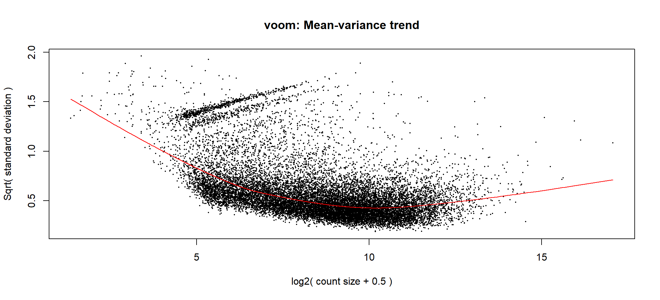

Voom transformation with observational weights

Version	Author	Date
d578f46	Ha Manh Tran	2023-01-21
159f352	tranmanhha135	2023-01-21
3119fad	tranmanhha135	2022-11-05

Observational & group level weights

# voom transformation with sample weights using full_design matrix for group-specific weights
voom1 <- limma::voomWithQualityWeights(counts = dge, design = full_design, plot = TRUE)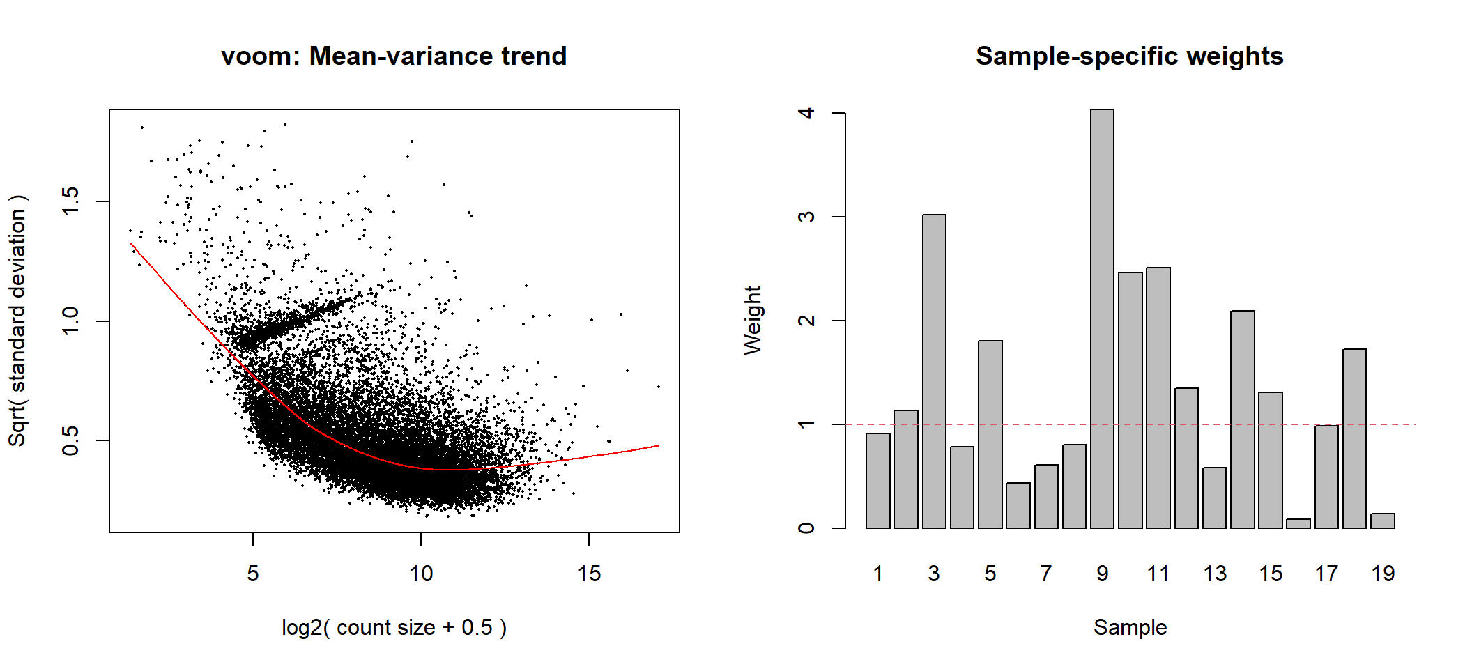

Voom transformation with observational and group-specific weights

Version	Author	Date
d578f46	Ha Manh Tran	2023-01-21
159f352	tranmanhha135	2023-01-21
3119fad	tranmanhha135	2022-11-05

Observational & sample level weights

# voom transformation with sample weights using null design matrix
voom2 <- limma::voomWithQualityWeights(counts = dge,design = null_design, plot = TRUE)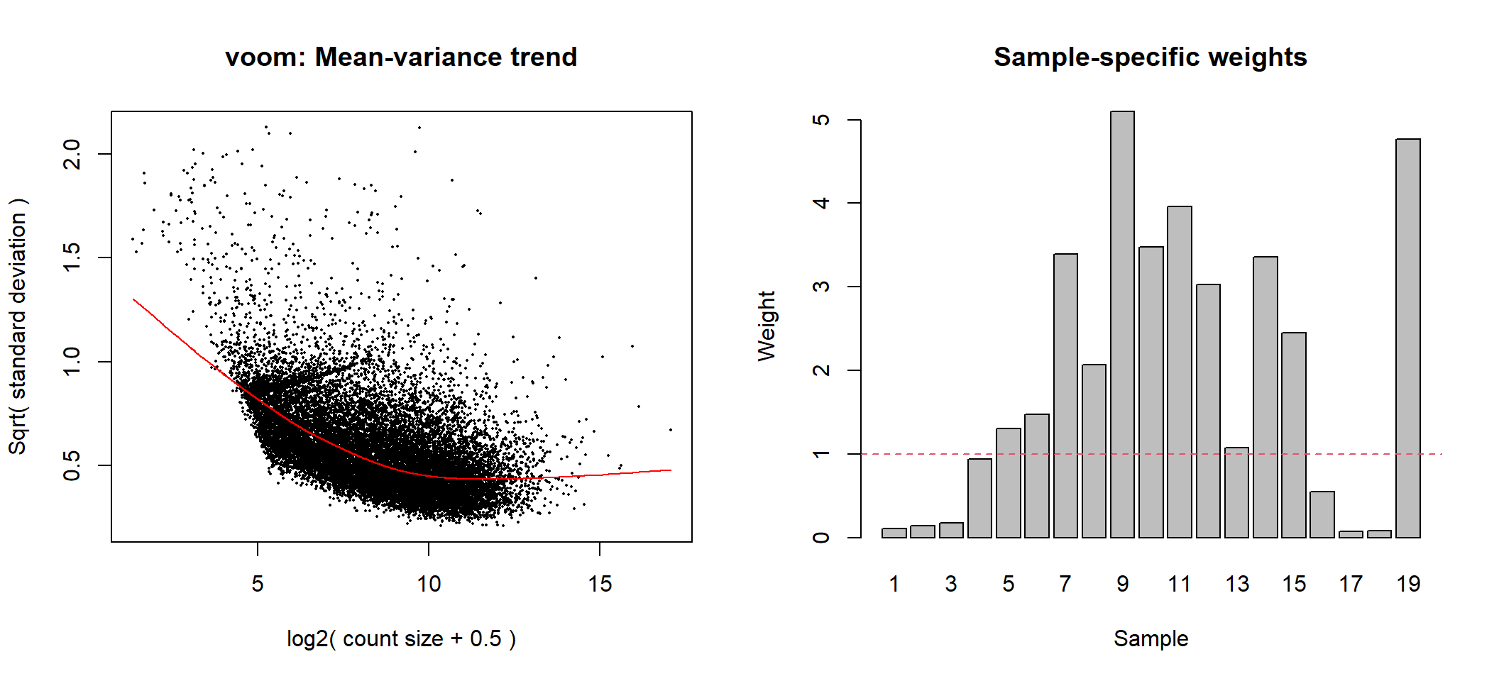

Voom transformation with observational and sample-specific weights

Version	Author	Date
d578f46	Ha Manh Tran	2023-01-21
159f352	tranmanhha135	2023-01-21
3119fad	tranmanhha135	2022-11-05

Apply linear model

Without FC cutoff and an FDR adj.p.val of 0.05, the INT vs CONT comparison still have nearly 2000 DE genes (TABLE 2). Thus, we can afford to be more stringent with our adjustment method and adj.p.val cutoff. Additionally, when the list of DE genes is large, we can apply a fold change cutoff through application of TREAT to prioritise the genes with greater fold changes and potentially more biologically relevant. Idealy, we are aiming for ~300 genes genes. Functional enrichment analysis with this number of genes should generate meaningful results.

Importantly, the FC threshold used in TREAT should be chosen as a small value below which results should be ignored, instead of a target fold-change. In general, a modest fold-change of 1.1 - 1.5 is recommended. However, it is more important to select a fold-change cutoff that generates a sufficiently small list of DE genes.

A fold-change value of 1.5 and FDR<0.05, generated a sufficiently small number of DE genes for the INT vs CONT comparison. This should be sufficient for functional enrichment analysis (TABLE 11).

# specifying FC of interest
options(digits = 6)
fc <- c(1.05, 1.1, 1.5)
lfc <- log(x = fc, 2)

Without TREAT

# function for applying linear model, generate decideTest table, and extract topTable
limmaFit_ebayes <- function(x, adjMethod, p.val, tableNum){
  lm <- limma::lmFit(object = x, design = full_design) %>%
    contrasts.fit(contrasts = contrast) %>%
    limma::eBayes()
  
  lm_dt <- decideTests(object = lm, adjust.method = adjMethod, p.value = p.val)
  print(knitr::kable(summary(lm_dt)
                      , caption = paste0("TABLE ",tableNum, ": Number of significant DE genes with '", adjMethod, "' adjusment method, and at a p-value/adj.p-value of ", p.val)) %>% 
    kable_styling(bootstrap_options = c("striped", "hover")))

  lm_all <- lapply(1:ncol(lm), function(y){
    limma::topTable(lm, coef = y, number = Inf, adjust.method = adjMethod) %>%
      dplyr::select(c("gene", "gene_name", "gene_biotype", "logFC", "AveExpr", "P.Value", "adj.P.Val", "description", "entrezid"))
    })
  names(lm_all) <- as.data.frame(contrast) %>% colnames()
  return(lm_all)
}

lm_voom2_pval0.01 <- limmaFit_ebayes(x = voom2, adjMethod = "none", p.val = 0.01, 1)

TABLE 1: Number of significant DE genes with ‘none’ adjusment method, and at a p-value/adj.p-value of 0.01
	INT vs CONT
Down	305
NotSig	14943
Up	1974

lm_voom2_fdr0.05 <- limmaFit_ebayes(x = voom2, adjMethod = "fdr", p.val = 0.05, 2)

TABLE 2: Number of significant DE genes with ‘fdr’ adjusment method, and at a p-value/adj.p-value of 0.05
	INT vs CONT
Down	134
NotSig	15484
Up	1604

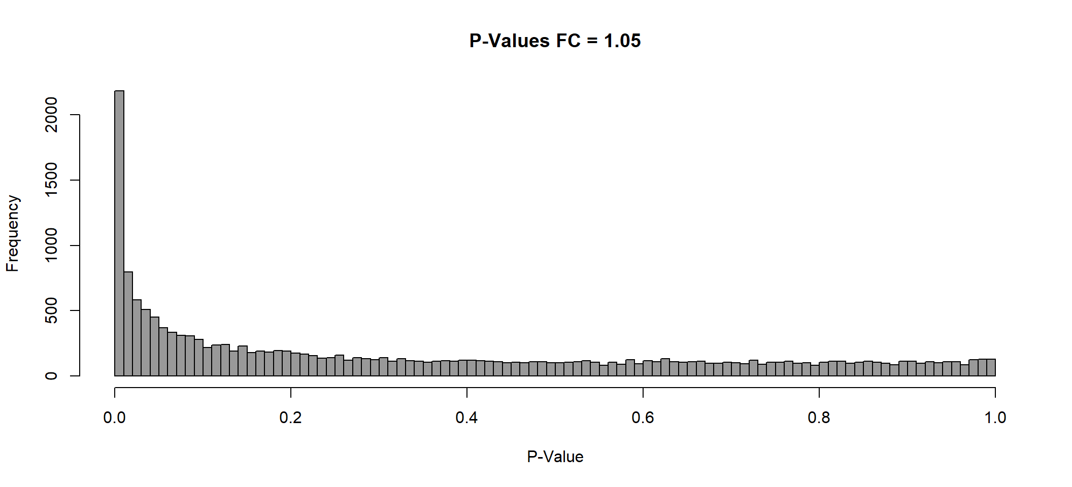
TREAT FC=1.05

limmaFit_treat <- function(x, fc, adjMethod, p.val, tableNum){
  lm_treat <- limma::lmFit(object = x, design = full_design) %>%
    contrasts.fit(contrasts = contrast) %>%
    limma::treat(fc = fc)
  
  lm_treat_dt <- decideTests(object = lm_treat, adjust.method = adjMethod, p.value = p.val)
  print(knitr::kable(summary(lm_treat_dt), 
                     caption = paste0("TABLE ", tableNum,": Number of DE genes significantly above a FC of ", fc, " with '", adjMethod, "' adjusment method, and at a p-value/adj.p-value of ", p.val)) %>% 
    kable_styling(bootstrap_options = c("striped", "hover")))
  
  lm_treat_all <- lapply(1:ncol(lm_treat), function(y){
    limma::topTreat(lm_treat, coef = y, number = Inf, adjust.method = adjMethod) %>%
      dplyr::select(c("gene", "gene_name", "gene_biotype", "logFC", "AveExpr", "P.Value", "adj.P.Val", "description", "entrezid"))
    })
  names(lm_treat_all) <- as.data.frame(contrast) %>% colnames()
  return(lm_treat_all)
}

assign(paste0("lmTreat_fc", fc[1], "_voom2_pval0.05"),
       limmaFit_treat(x = voom2, fc = fc[1], adjMethod = "none", p.val = 0.05, 3))

TABLE 3: Number of DE genes significantly above a FC of 1.05 with ‘none’ adjusment method, and at a p-value/adj.p-value of 0.05
	INT vs CONT
Down	1443
NotSig	12700
Up	3079

assign(paste0("lmTreat_fc", fc[1], "_voom2_pval0.01"),
       limmaFit_treat(x = voom2, fc = fc[1], adjMethod = "none", p.val = 0.01, 4))

TABLE 4: Number of DE genes significantly above a FC of 1.05 with ‘none’ adjusment method, and at a p-value/adj.p-value of 0.01
	INT vs CONT
Down	260
NotSig	15041
Up	1921

assign(paste0("lmTreat_fc", fc[1], "_voom2_fdr0.05"),
       limmaFit_treat(x = voom2, fc = fc[1], adjMethod = "fdr", p.val = 0.05, 5))

TABLE 5: Number of DE genes significantly above a FC of 1.05 with ‘fdr’ adjusment method, and at a p-value/adj.p-value of 0.05
	INT vs CONT
Down	95
NotSig	15593
Up	1534

TREAT FC=1.1

assign(paste0("lmTreat_fc", fc[2], "_voom2_pval0.05"),
       limmaFit_treat(x = voom2, fc = fc[2], adjMethod = "none", p.val = 0.05, 6))

TABLE 6: Number of DE genes significantly above a FC of 1.1 with ‘none’ adjusment method, and at a p-value/adj.p-value of 0.05
	INT vs CONT
Down	1230
NotSig	13070
Up	2922

assign(paste0("lmTreat_fc", fc[2], "_voom2_pval0.01"),
       limmaFit_treat(x = voom2, fc = fc[2], adjMethod = "none", p.val = 0.01, 7))

TABLE 7: Number of DE genes significantly above a FC of 1.1 with ‘none’ adjusment method, and at a p-value/adj.p-value of 0.01
	INT vs CONT
Down	187
NotSig	15205
Up	1830

assign(paste0("lmTreat_fc", fc[2], "_voom2_fdr0.05"),
       limmaFit_treat(x = voom2, fc = fc[2], adjMethod = "fdr", p.val = 0.05, 8))

TABLE 8: Number of DE genes significantly above a FC of 1.1 with ‘fdr’ adjusment method, and at a p-value/adj.p-value of 0.05
	INT vs CONT
Down	55
NotSig	15775
Up	1392

TREAT FC=1.5

assign(paste0("lmTreat_fc", fc[3], "_voom2_pval0.05"),
       limmaFit_treat(x = voom2, fc = fc[3], adjMethod = "none", p.val = 0.05, 9))

TABLE 9: Number of DE genes significantly above a FC of 1.5 with ‘none’ adjusment method, and at a p-value/adj.p-value of 0.05
	INT vs CONT
Down	155
NotSig	15317
Up	1750

assign(paste0("lmTreat_fc", fc[3], "_voom2_pval0.01"),
       limmaFit_treat(x = voom2, fc = fc[3], adjMethod = "none", p.val = 0.01, 10))

TABLE 10: Number of DE genes significantly above a FC of 1.5 with ‘none’ adjusment method, and at a p-value/adj.p-value of 0.01
	INT vs CONT
Down	14
NotSig	16238
Up	970

assign(paste0("lmTreat_fc", fc[3], "_voom2_fdr0.05"),
       limmaFit_treat(x = voom2, fc = fc[3], adjMethod = "fdr", p.val = 0.05, 11))

TABLE 11: Number of DE genes significantly above a FC of 1.5 with ‘fdr’ adjusment method, and at a p-value/adj.p-value of 0.05
	INT vs CONT
Down	2
NotSig	16834
Up	386

Differential Gene Expression analysis

For the Intact vs Control comparison, a rigorous statistical test was used to reduce the list of DE genes down to a more biologically relevant number. This included testing significance relative to a fold change threshold (TREAT). For this comparison, genes significantly above of FC of 1.01, 1.1, and 1.5 and FDR < 0.05 are visualised.

Although only DE genes significantly above a fold-change value of 1.5 and FDR<0.05 will be used for functional enrichment analysis, visualisations for other cut-off are retained for data exploratory purposes.

### Old code used to iteratively generate lmTreat dataset with different fc cutoff
## with treat
lmTreat <- list()
lmTreat_dt <- list()
lmTreat_all <- list()
lmTreat_sig <- list()

for (i in 1:length(fc)) {
  x <- fc[i] %>% as.character()
  lmTreat[[x]] <- limma::lmFit(object = voom2, design = full_design) %>%
    limma::contrasts.fit(contrasts = contrast) %>%
    limma::treat(lfc = lfc[i])

  # decide test, do before taking topTreat, as input need to be MArraryLM list
  lmTreat_dt[[x]] <- decideTests(lmTreat[[x]], adjust.methods = "fdr", p.value = 0.05)

  # extract a table of genes from a linear model fit, export and used for downstream analysis
  lmTreat_all[[x]] <- topTreat(fit = lmTreat[[x]], coef = 1, number = Inf, adjust.method = "fdr") %>%
    dplyr::select(c("gene_name", "logFC", "AveExpr", "P.Value", "adj.P.Val", "description", "entrezid"))

  # extract a table of significant genes from a linear model fit, export and used for downstream analysis
  lmTreat_sig[[x]] <- topTreat(fit = lmTreat[[x]], coef = 1, number = Inf, adjust.method = "fdr", p.value = 0.05) %>%
    dplyr::select(c("gene_name", "logFC", "AveExpr", "P.Value", "adj.P.Val", "description", "entrezid"))
}

TREAT FC= 1.05

P Value histogram

lmTreat_hist <- list()
for (i in 1:length(fc)) {
  x <- fc[i] %>% as.character()
  lmTreat_hist[[x]] <- hist(x = lmTreat[[x]]$p.value, breaks = 100, plot = F) 
}
plot(
  x = lmTreat_hist[[1]],
  main = paste0("P-Values FC = ", fc[[1]]),
  xlab = "P-Value",
  col = "gray60"
)

Version	Author	Date
d578f46	Ha Manh Tran	2023-01-21
159f352	tranmanhha135	2023-01-21
3119fad	tranmanhha135	2022-11-05

invisible(dev.print(svg, here::here(paste0("2_plots/de/pval_", fc[1], ".svg"))))

MA Plot

ma <- list()
for (i in 1:length(fc)) {
  x <- fc[i] %>% as.character()
  
  # add an extra column and determine whether the DE genes are significant
  lmTreat_all[[x]] <- lmTreat_all[[x]] %>%
    as.data.frame() %>%
    dplyr::mutate(Expression = case_when(
      adj.P.Val <= 0.05 & logFC >= lfc ~ "Up-regulated",
      adj.P.Val <= 0.05 & logFC <= -lfc ~ "Down-regulated",
      TRUE ~ "Insignificant"
    ))

  # adding labels to top genes
  top <- 3
  top_limma <- bind_rows(
    lmTreat_all[[x]] %>%
      dplyr::filter(Expression == "Up-regulated") %>%
      arrange(adj.P.Val, desc(abs(logFC))) %>%
      head(top),
    lmTreat_all[[x]] %>%
      dplyr::filter(Expression == "Down-regulated") %>%
      arrange(adj.P.Val, desc(abs(logFC))) %>%
      head(top)
  )
  invisible(top_limma %>% as.data.frame())

  ma[[x]] <- lmTreat_all[[x]] %>%
    ggplot(aes(x = AveExpr, y = logFC)) +
    geom_point(aes(colour = Expression),

      ### PUBLISH
      size = 1.5,
      # alpha = 0.7,
      show.legend = T
    ) +
    # geom_label_repel(
    #   data = top_limma,
    #   mapping = aes(x = AveExpr, logFC, label = gene_name),
    # 
    #   ### PUBLISH
    #   size = 1.7,
    #   label.padding = 0.15,
    #   # label.r = 0.15,
    #   box.padding = 0.15
    #   # point.padding = 0.2
    # ) +
    geom_hline(yintercept = c(-fc[i], 0, fc[i]), linetype = c("dashed", "solid", "dashed")) +

    ### PUBLISH
    ylim(-8, 8) +
    theme(legend.position = "bottom",
          legend.box.margin = margin(-10,0,0,0),
          legend.key.size = unit(0, "lines")
          )+

    xlab(expression("log"[2] * "CPM")) +
    ylab(expression("log"[2] * "FC")) +
    scale_fill_manual(values = c("dodgerblue3", alpha(colour = "gray80", alpha = 0.9), "firebrick3")) +
    scale_color_manual(labels = c(paste0("Down: ", sum(lmTreat_all[[x]]$Expression == "Down-regulated"), "  "),
                                  paste0("NS: ", sum(lmTreat_all[[x]]$Expression == "Insignificant"), "  "),
                                  paste0("Up: ", sum(lmTreat_all[[x]]$Expression == "Up-regulated"), " ")), 
                       values = c("dodgerblue3", alpha(colour = "gray80", alpha = 0.6), "firebrick3")) +
    
    guides(colour = guide_legend(override.aes = list(size = 1.5))) +
    labs(
      # title = "MA Plot: LIMMA-VOOM + TREAT",
      # subtitle = "Intact vs Control",
      colour = "Expression")

  # save to directory
  ggsave(paste0("ma_", fc[i], ".png"),
         plot = ma[[x]] + pub + theme(
           legend.position = "bottom",
           legend.box.margin = margin(-10, 0, 0, 0),
           legend.key.size = unit(0, "lines")
         ),
         path = here::here("2_plots/de/"),
         width = 250,
         height = 166,
         units = "mm",
         dpi = 800
  )
}

# display
ma[[1]]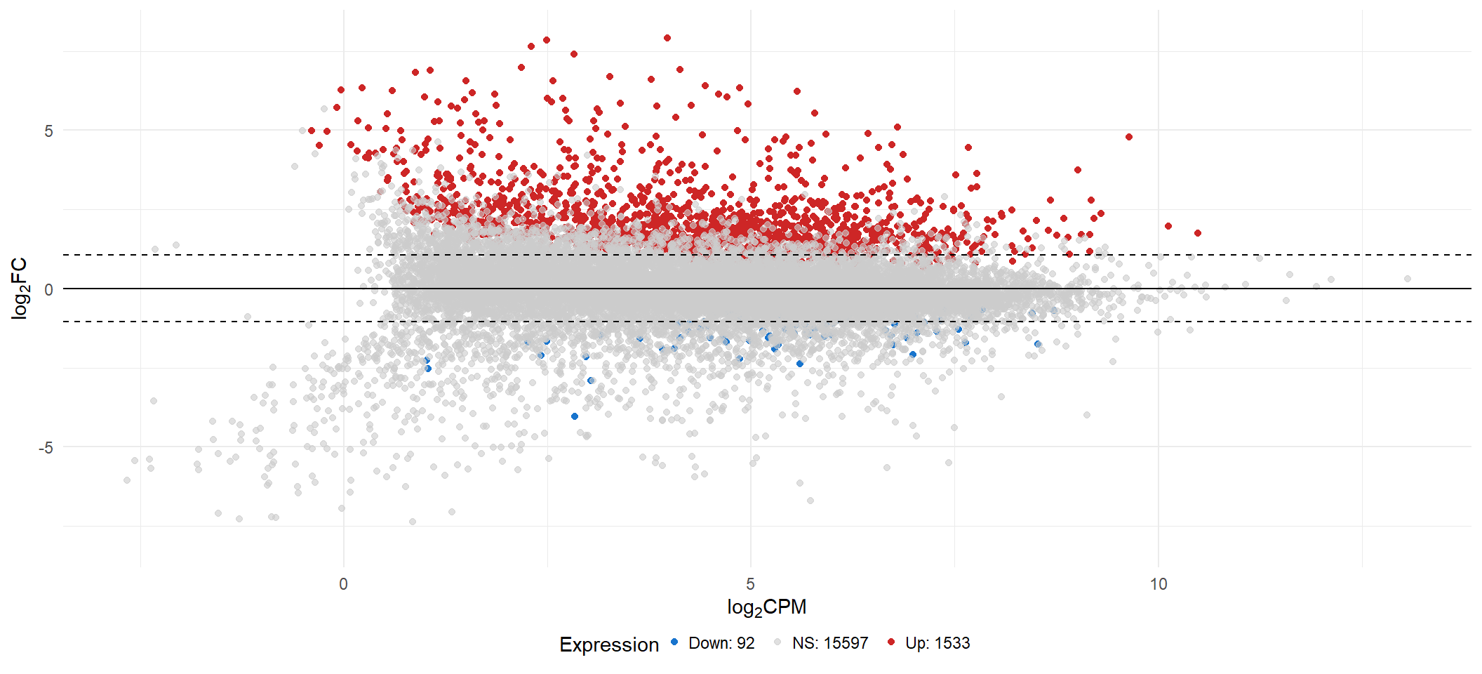

Version	Author	Date
b44640a	Ha Manh Tran	2023-01-23
d578f46	Ha Manh Tran	2023-01-21
159f352	tranmanhha135	2023-01-21
4d51a4e	tranmanhha135	2023-01-20
3119fad	tranmanhha135	2022-11-05

Volcano Plot

vol <- list()
for (i in 1:length(fc)) {
  x <- fc[i] %>% as.character()

  # adding labels to top genes
  top <- 3
  top_limma <- bind_rows(
    lmTreat_all[[x]] %>%
      dplyr::filter(Expression == "Up-regulated") %>%
      arrange(adj.P.Val, desc(abs(logFC))) %>%
      head(top),
    lmTreat_all[[x]] %>%
      dplyr::filter(Expression == "Down-regulated") %>%
      arrange(adj.P.Val, desc(abs(logFC))) %>%
      head(top)
  )
  invisible(top_limma %>% as.data.frame())

  # generate vol plot with the allDEgene data.frame
  vol[[x]] <- lmTreat_all[[x]] %>%
    ggplot(aes(
      x = logFC,
      y = -log(adj.P.Val, 10)
    )) +
    geom_point(aes(colour = Expression),

      ### PUBLISH
      size = 1.5,
      # alpha = 0.8,
      show.legend = T
    ) +
    # geom_label_repel(
    #   data = top_limma,
    #   mapping = aes(logFC, -log(adj.P.Val, 10), label = gene_name),
    # 
    #   ### PUBLISH
    #   size = 1.7,
    #   label.padding = 0.15,
    #   # label.r = 0.15,
    #   box.padding = 0.15
    #   # point.padding = 0.2
    # ) +

    ### PUBLISH
    xlim(-8.15, 8.15)+
    theme(legend.position = "bottom",
          legend.box.margin = margin(-10,0,0,0),
          legend.key.size = unit(0, "lines")
          )+

    xlab(expression("log"[2] * "FC")) +
    ylab(expression("-log"[10] * "FDR")) +
    scale_fill_manual(values = c("dodgerblue3", alpha(colour = "gray80", alpha = 0.9), "firebrick3")) +
    scale_color_manual(labels = c(paste0("Down: ", sum(lmTreat_all[[x]]$Expression == "Down-regulated"), "  "),
                                  paste0("NS: ", sum(lmTreat_all[[x]]$Expression == "Insignificant"), "  "),
                                  paste0("Up: ", sum(lmTreat_all[[x]]$Expression == "Up-regulated"), " ")), 
                       values = c("dodgerblue3", alpha(colour = "gray80", alpha = 0.6), "firebrick3")) +   
    
    guides(colour = guide_legend(override.aes = list(size = 1.5))) +
    labs(

      ### PUBLISH
      # title = "Volcano Plot: LIMMA-VOOM + TREAT",
      # subtitle = "Intact vs Control",
      colour = "Expression"
    )

  # save to directory
  ggsave(paste0("vol_", fc[i], ".png"),
         plot = vol[[x]] + pub + theme(
           legend.position = "bottom",
           legend.box.margin = margin(-10, 0, 0, 0),
           legend.key.size = unit(0, "lines")
         ),
         path = here::here("2_plots/de/"),
         width = 250,
         height = 166,
         units = "mm",
         dpi = 800
  )
}

# display
vol[[1]]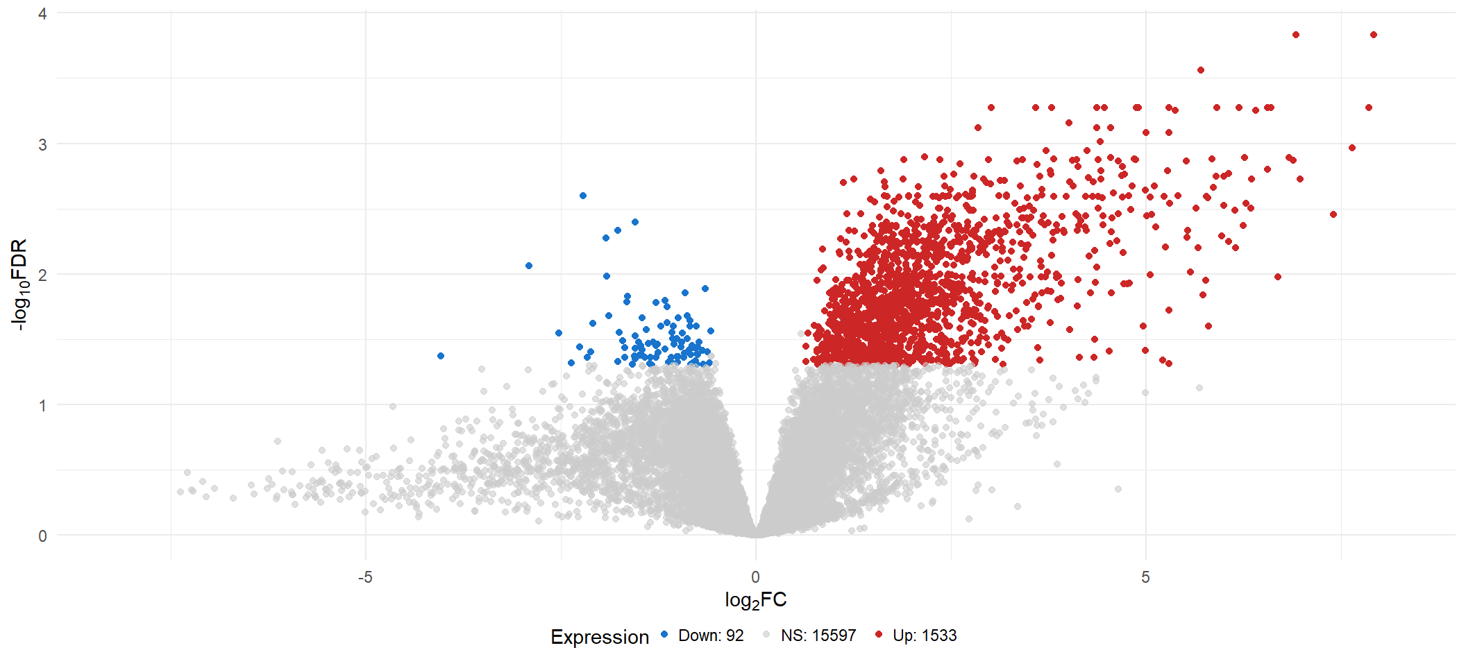

Version	Author	Date
b44640a	Ha Manh Tran	2023-01-23
d578f46	Ha Manh Tran	2023-01-21
159f352	tranmanhha135	2023-01-21
3119fad	tranmanhha135	2022-11-05

Top Upregulated

# create df with normalised read counts with an additional entrezid column for binding
logCPM <- cpm(dge, prior.count = 3, log = TRUE) %>% subset(select = 1:7)
rownames(logCPM) <- dge$genes$gene_name
# colnames(logCPM) <- c("Control 1", "Control 2", "Control 4", "Intact 1", "Intact 2", "Intact 3", "Intact 4")

# colour palette for heatmap
my_palette <- colorRampPalette(c("dodgerblue3", "white", "firebrick3"))(n = 201)

# df for heatmap annotation of sample group
anno <- as.factor(dge$samples$group) %>% as.data.frame() %>% dplyr::slice(1:7)
colnames(anno) <- "Sample Groups"
anno$`Sample Groups` <- gsub("CONT", "Control", anno$`Sample Groups`)
anno$`Sample Groups` <- gsub("INT", "Intact", anno$`Sample Groups`)
rownames(anno) <- colnames(logCPM)

# setting colour of sample group annotation
anno_colours <- c("#f8766d", "#a3a500")
names(anno_colours) <- c("Control", "Intact")

logCPM_up=list()
logCPM_down=list()
for (i in 1:length(fc)) {
  x <- fc[i] %>% as.character()
  
  # filtering top unregulated genes then filter the logCPM values of those genes.
  upReg <- lmTreat_sig[[x]] %>%
    dplyr::filter(logFC > 0) %>%
    arrange(sort(adj.P.Val, decreasing = F))
  upReg <- upReg[1:20,]
  logCPM_up[[x]] <- logCPM[upReg$gene_name,] %>% as.data.frame()
  

  # filtering top unregulated genes then filter the logCPM values of those genes.
  downReg <- lmTreat_sig[[x]] %>%
    dplyr::filter(logFC < 0) %>%
    arrange(sort(adj.P.Val, decreasing = F))
  if (nrow(downReg) >= 20) {max <-  20} else {max <-  nrow(downReg)}
  downReg <- downReg[1:max,]
  logCPM_down[[x]] <- logCPM[downReg$gene_name,] %>% as.data.frame()
}

heat_up=list()

my_palette <- colorRampPalette(c(
  rgb(32,121,226, maxColorValue = 255),
  # rgb(144,203,180, maxColorValue = 255), 
  rgb(254,248,239, maxColorValue = 255), 
  # rgb(251,192,52, maxColorValue = 255), 
  rgb(226,46,45, maxColorValue = 255)))(n = 201)

for (i in 1:length(fc)) {
  x <- fc[i] %>% as.character()
  heat_up[[x]] <-
    pheatmap(
      mat = logCPM_up[[x]], 
  
      ### Publish
      show_colnames = F,
      main = paste0("Top ", nrow(logCPM_up[[x]]), " significant upregulated genes\n"),
      legend = F,
      annotation_legend = T,
      fontsize = 8,
      fontsize_col = 9,
      fontsize_number = 7,
      fontsize_row = 8,
      treeheight_row = 25,
      treeheight_col = 10,
      clustering_distance_rows = "euclidean",
      legend_breaks = c(seq(-3, 11, by = .5), 1.3),
      legend_labels = c(seq(-3, 11, by = .5), "Z-Score"),
      angle_col = 90,
      cutree_cols = 2,
      cutree_rows = 1,
      border_color = NA,
      color = my_palette,
      scale = "row",
      annotation_col = anno,
      annotation_colors = list("Sample Groups" = anno_colours),
      annotation_names_col = F,
      annotation = T,
      silent = T,
      
      labels_row = as.expression(lapply(rownames(logCPM_up[[x]]), function(a) bquote(italic(.(a)))))
      
  ) %>% as.ggplot()
  
# save to directory
  ggsave(paste0("heat_up_", fc[i], ".svg"),
         plot = heat_up[[x]],
         path = here::here("2_plots/de/"),
         width = 166,
         height = 200,
         units = "mm"
  )
}

heat_up[[1]]

Version	Author	Date
d578f46	Ha Manh Tran	2023-01-21
159f352	tranmanhha135	2023-01-21
691cf34	Ha Manh Tran	2023-01-20
3119fad	tranmanhha135	2022-11-05

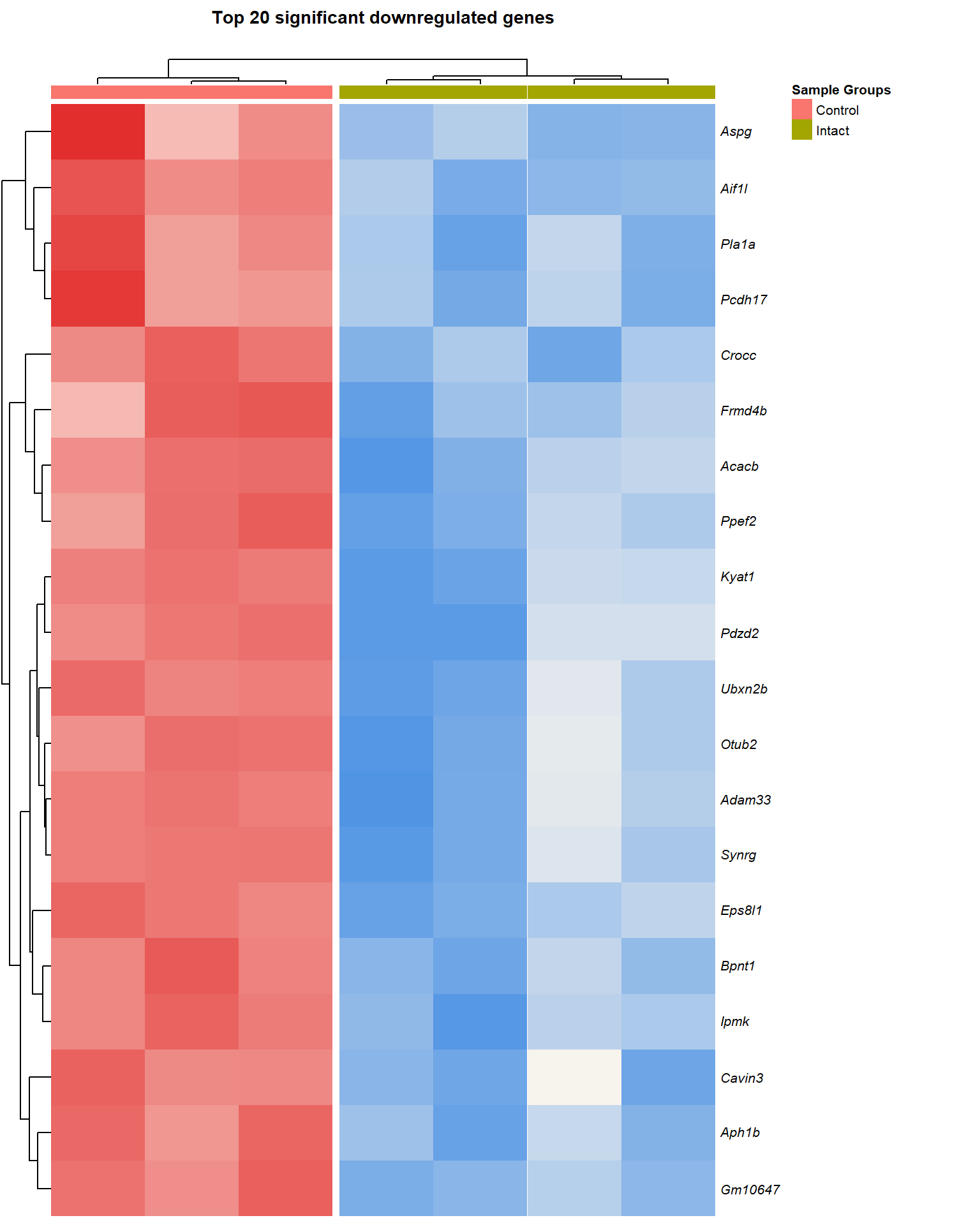
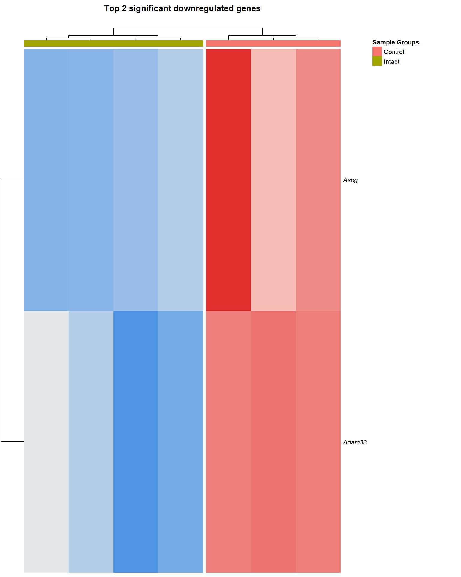
Top Downregulated

heat_down=list()
for (i in 1:length(fc)) {
  x <- fc[i] %>% as.character()
  heat_down[[x]] <-
    pheatmap(
      mat = logCPM_down[[x]],
  
      ### Publish
      show_colnames = F,
      main = paste0("Top ", nrow(logCPM_down[[x]]), " significant downregulated genes\n"),
      legend = F,
      annotation_legend = T,
      fontsize = 8,
      fontsize_col = 9,
      fontsize_number = 7,
      fontsize_row = 8,
      treeheight_row = 25,
      treeheight_col = 10,
      clustering_distance_rows = "euclidean",
      legend_breaks = c(seq(-3, 11, by = .5), 1.3),
      legend_labels = c(seq(-3, 11, by = .5), "Z-Score"),
      angle_col = 90,
      cutree_cols = 2,
      cutree_rows = 1,
      border_color = NA,
      color = my_palette,
      scale = "row",
      annotation_col = anno,
      annotation_colors = list("Sample Groups" = anno_colours),
      annotation_names_col = F,
      annotation = T,
      silent = T,
      
      labels_row = as.expression(lapply(rownames(logCPM_down[[x]]), function(a) bquote(italic(.(a)))))

  ) %>% as.ggplot()
  
# save to directory
   ggsave(paste0("heat_down_", fc[i], ".svg"),
         plot = heat_down[[x]],
         path = here::here("2_plots/de/"),
         width = 166,
         height = 200,
         units = "mm"
  )
}

heat_down[[1]]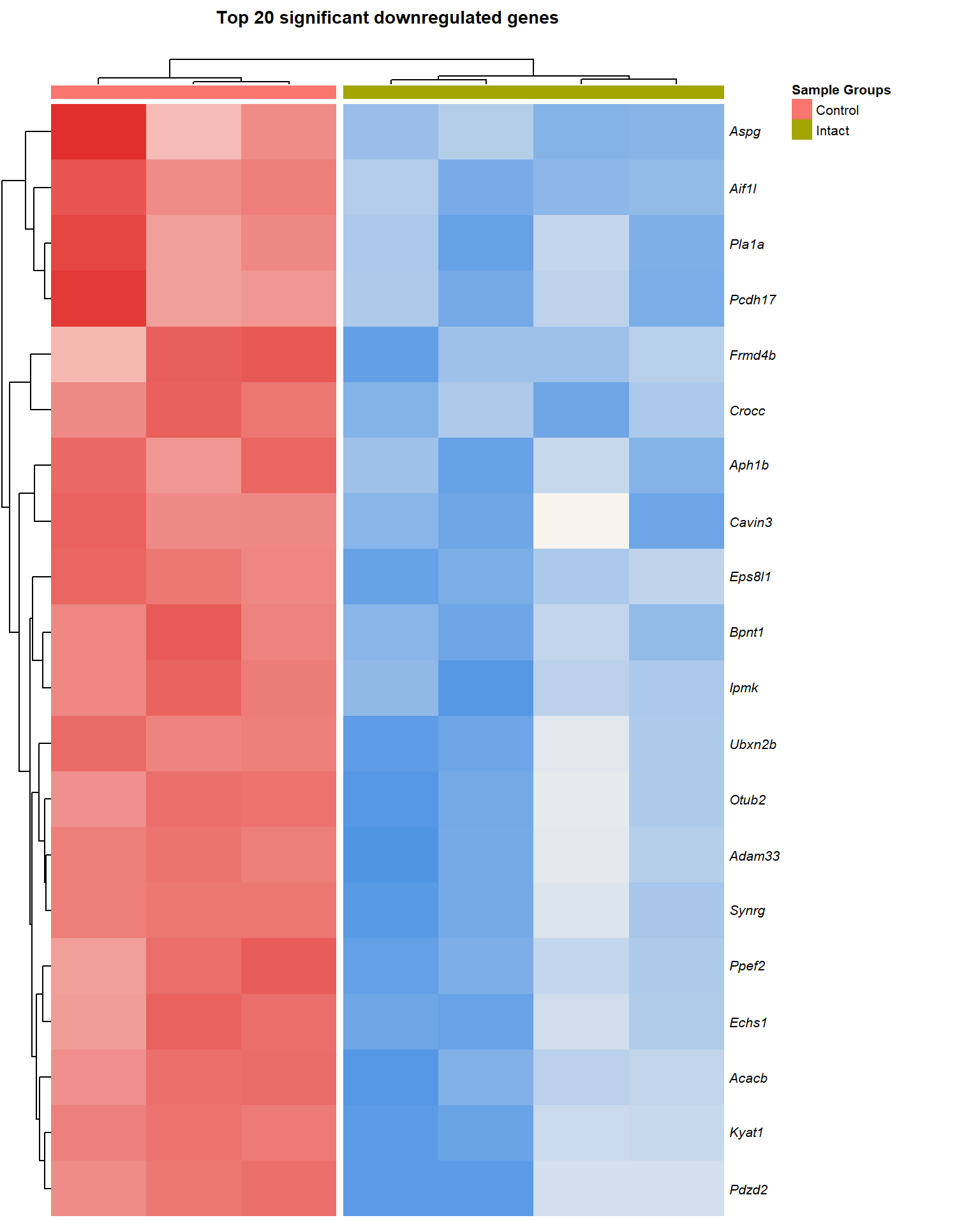

Version	Author	Date
d578f46	Ha Manh Tran	2023-01-21
159f352	tranmanhha135	2023-01-21
691cf34	Ha Manh Tran	2023-01-20
3119fad	tranmanhha135	2022-11-05

TREAT FC= 1.1

P Value histogram

plot(x = lmTreat_hist[[2]],
     main = paste0("P-Values FC = ", fc[[2]]),
     xlab = "P-Value",
     col = "gray60")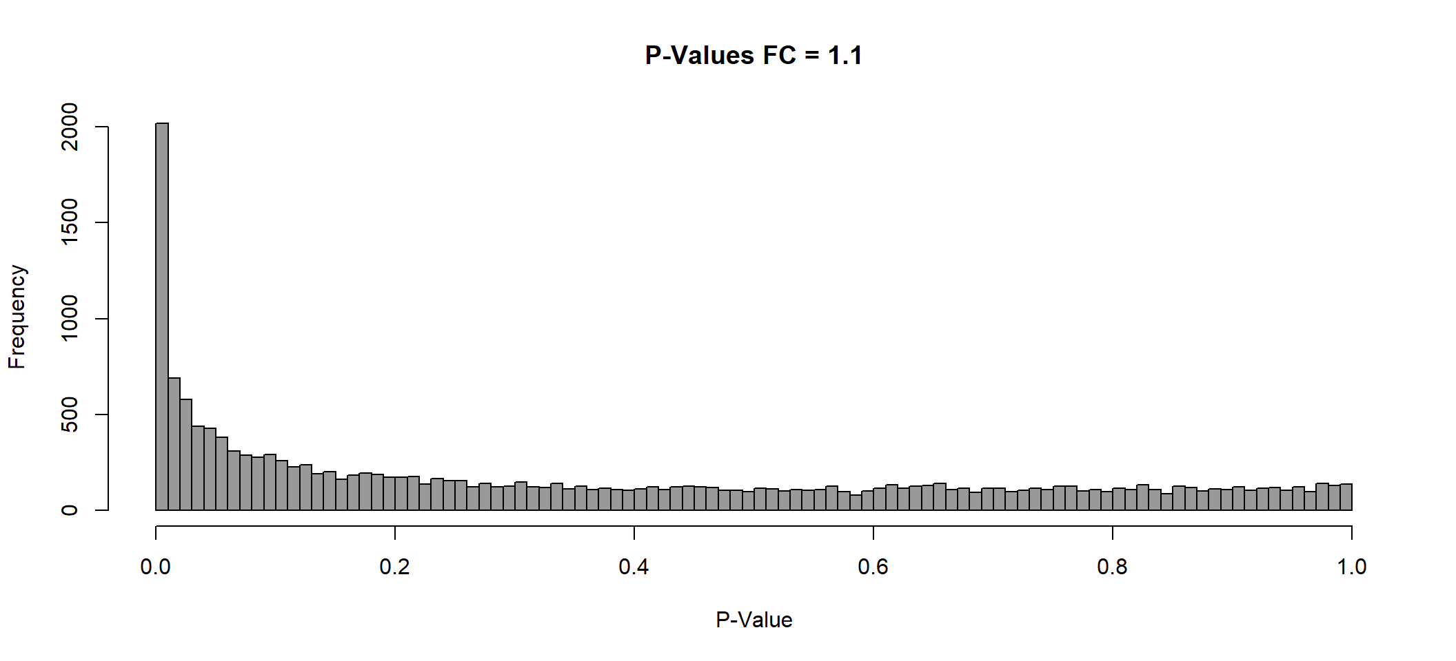

Version	Author	Date
d578f46	Ha Manh Tran	2023-01-21
159f352	tranmanhha135	2023-01-21
691cf34	Ha Manh Tran	2023-01-20
3119fad	tranmanhha135	2022-11-05

invisible(dev.print(svg, here::here(paste0("2_plots/de/pval_", fc[2], ".svg"))))

MA Plot

ma[[2]]

Version	Author	Date
b44640a	Ha Manh Tran	2023-01-23
d578f46	Ha Manh Tran	2023-01-21
159f352	tranmanhha135	2023-01-21
4d51a4e	tranmanhha135	2023-01-20
691cf34	Ha Manh Tran	2023-01-20
3119fad	tranmanhha135	2022-11-05

Volcano Plot

vol[[2]]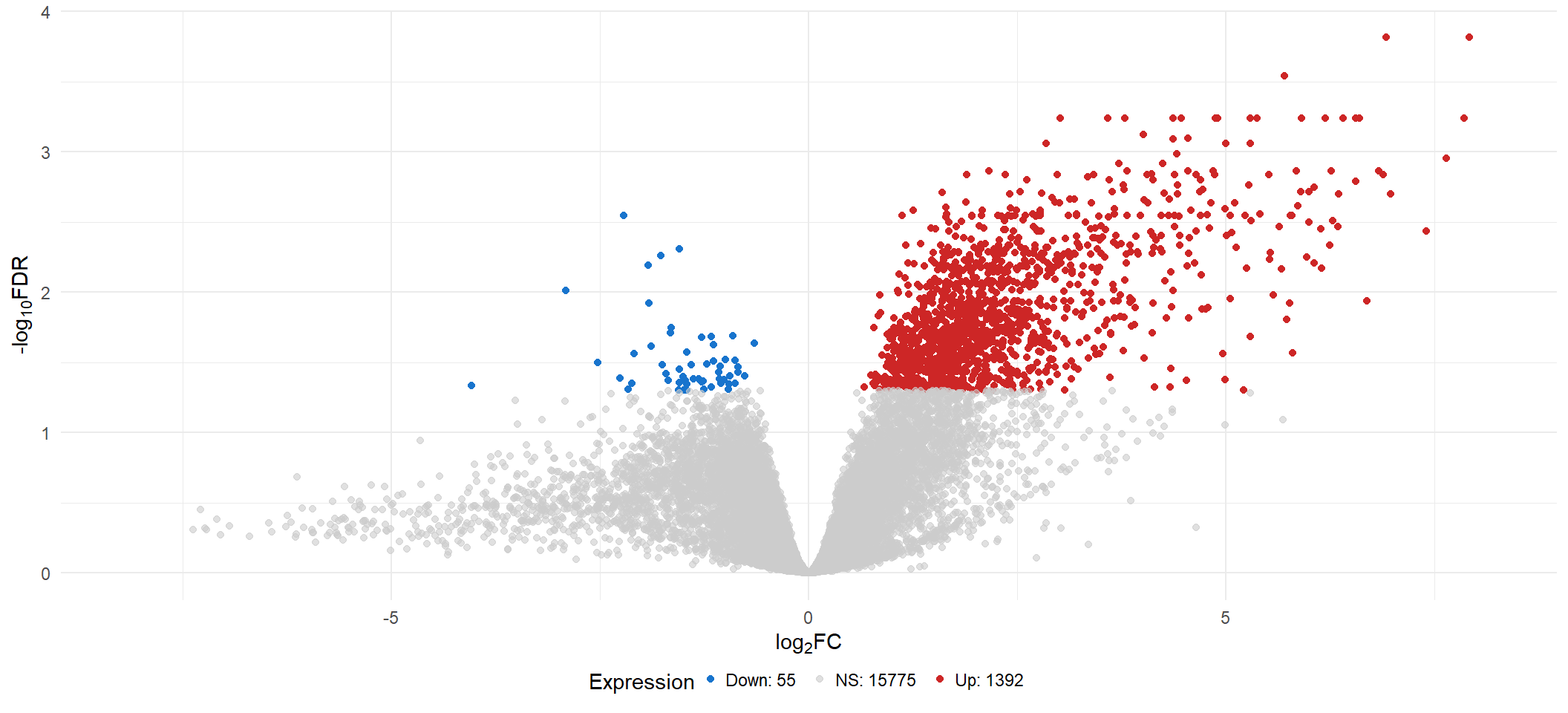

Version	Author	Date
b44640a	Ha Manh Tran	2023-01-23
d578f46	Ha Manh Tran	2023-01-21
159f352	tranmanhha135	2023-01-21
691cf34	Ha Manh Tran	2023-01-20
3119fad	tranmanhha135	2022-11-05

Top Upregulated

heat_up[[2]]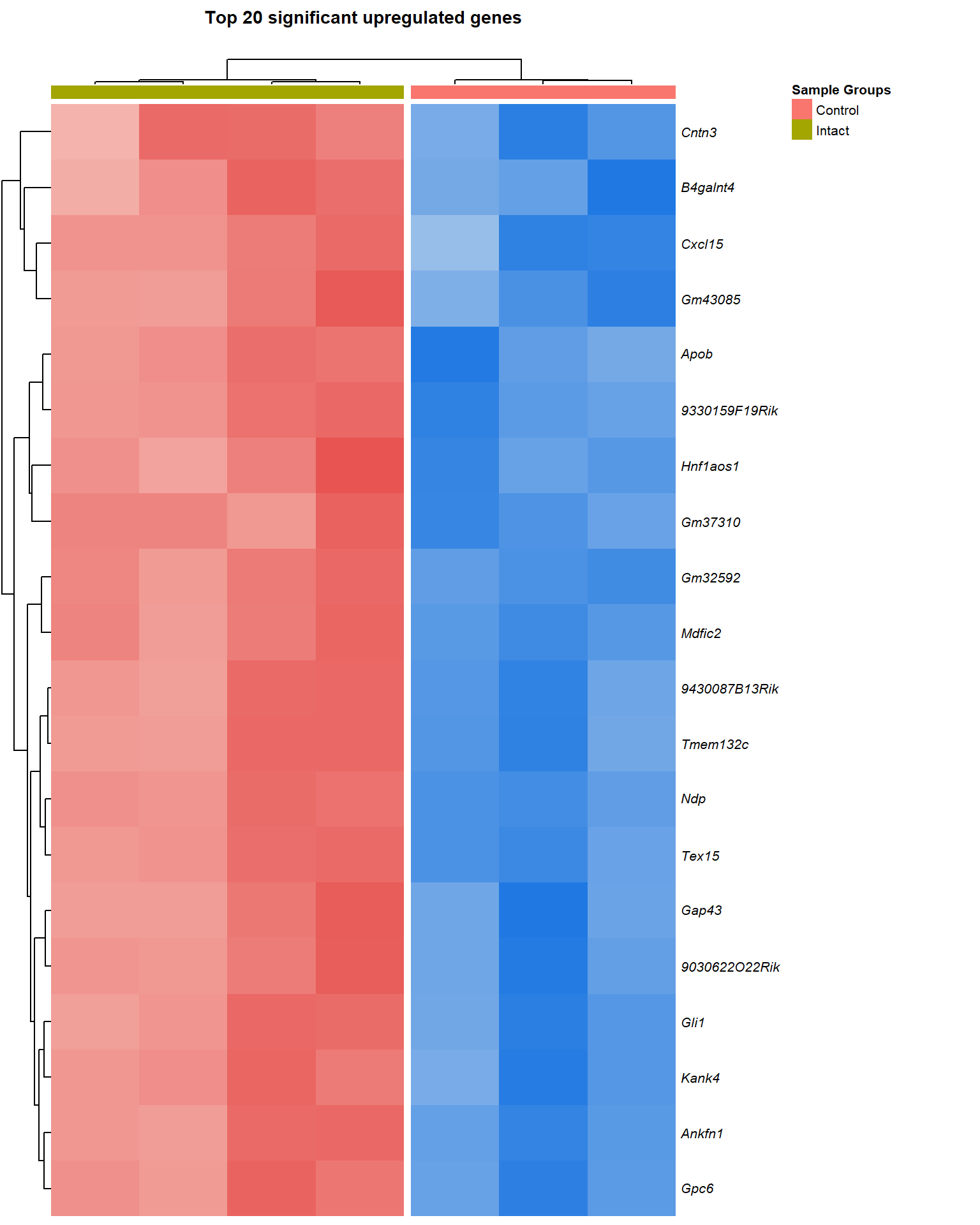

Version	Author	Date
d578f46	Ha Manh Tran	2023-01-21
159f352	tranmanhha135	2023-01-21
691cf34	Ha Manh Tran	2023-01-20
3119fad	tranmanhha135	2022-11-05

Top Downregulated

heat_down[[2]]

Version	Author	Date
d578f46	Ha Manh Tran	2023-01-21
159f352	tranmanhha135	2023-01-21
691cf34	Ha Manh Tran	2023-01-20
3119fad	tranmanhha135	2022-11-05

TREAT FC= 1.5

P Value histogram

plot(x = lmTreat_hist[[3]],
     main = paste0("P-Values FC = ", fc[[3]]),
     xlab = "P-Value",
     col = "gray60")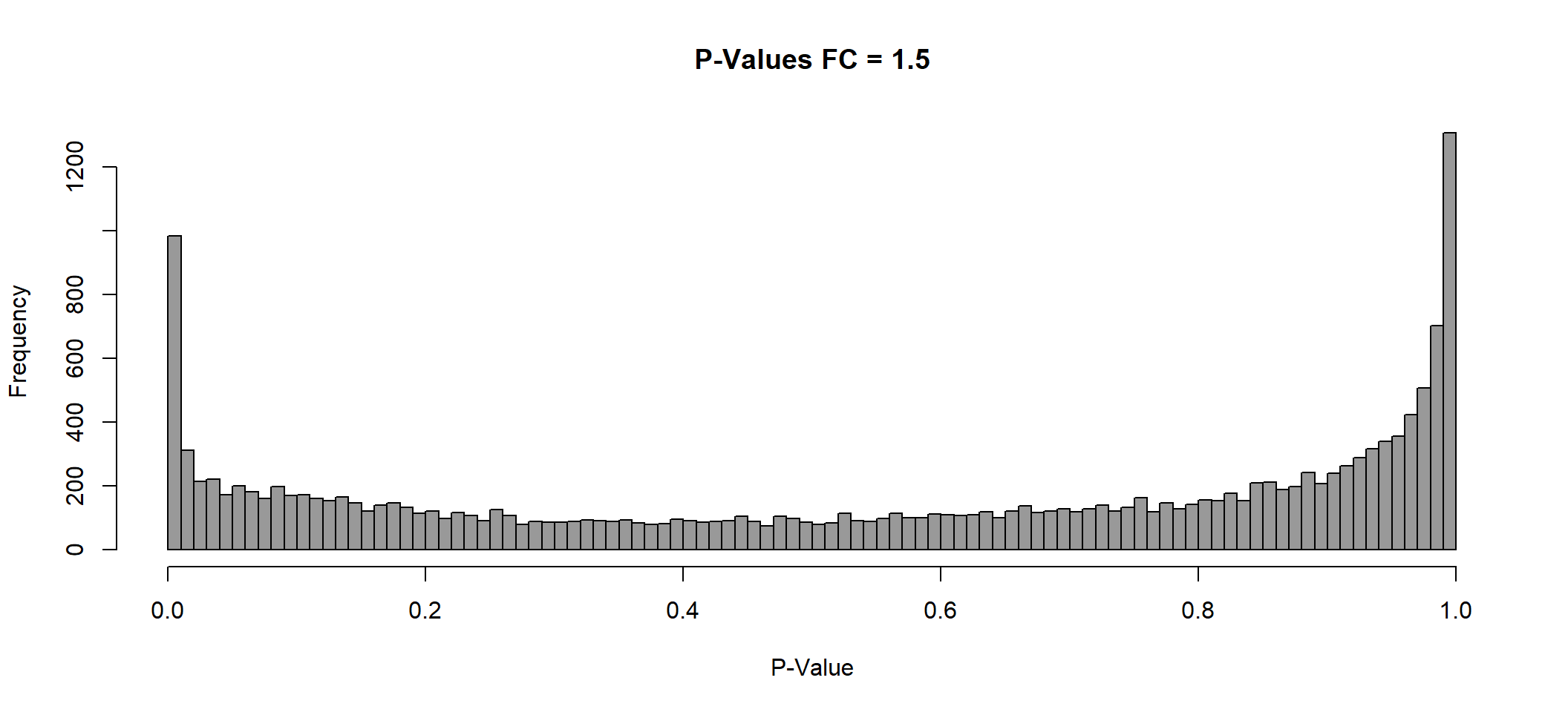

Version	Author	Date
d578f46	Ha Manh Tran	2023-01-21
159f352	tranmanhha135	2023-01-21
3119fad	tranmanhha135	2022-11-05

invisible(dev.print(svg, here::here(paste0("2_plots/de/pval_", fc[3], ".svg"))))

MA Plot

ma[[3]]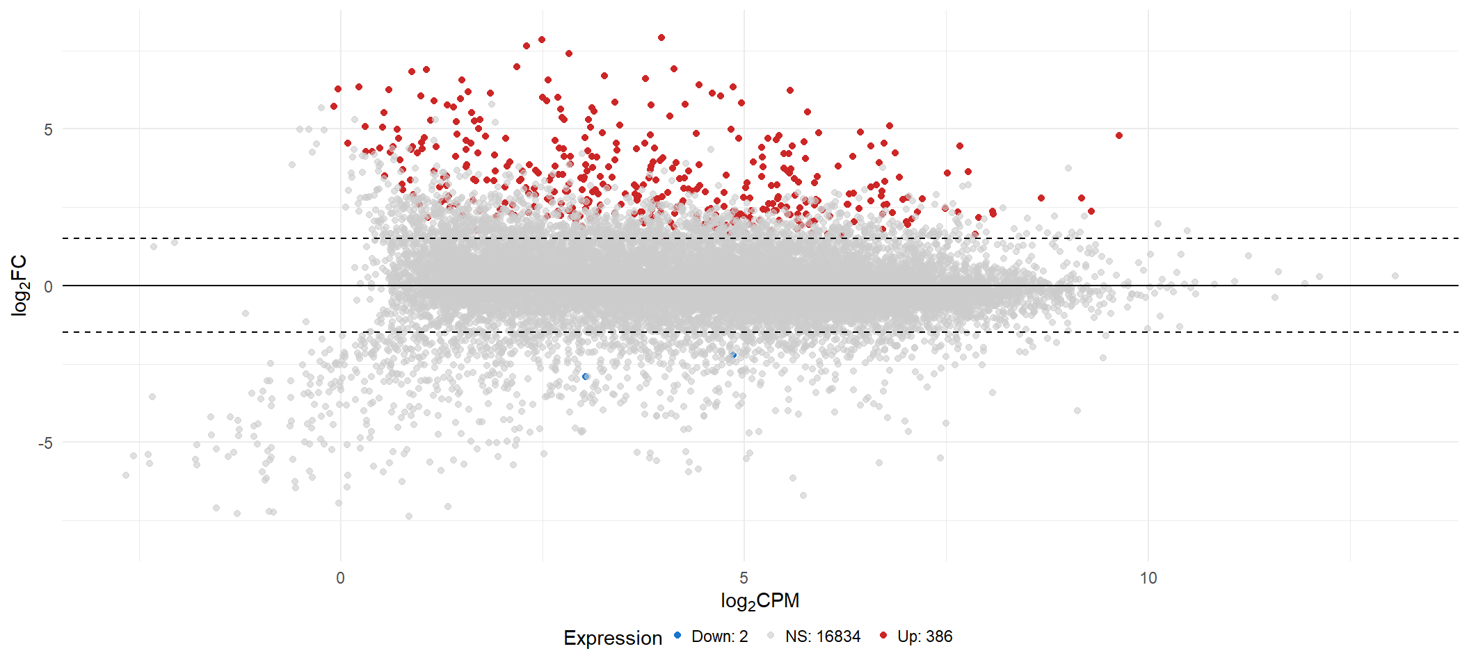

Version	Author	Date
b44640a	Ha Manh Tran	2023-01-23
d578f46	Ha Manh Tran	2023-01-21
159f352	tranmanhha135	2023-01-21
4d51a4e	tranmanhha135	2023-01-20
3119fad	tranmanhha135	2022-11-05

Volcano Plot

vol[[3]]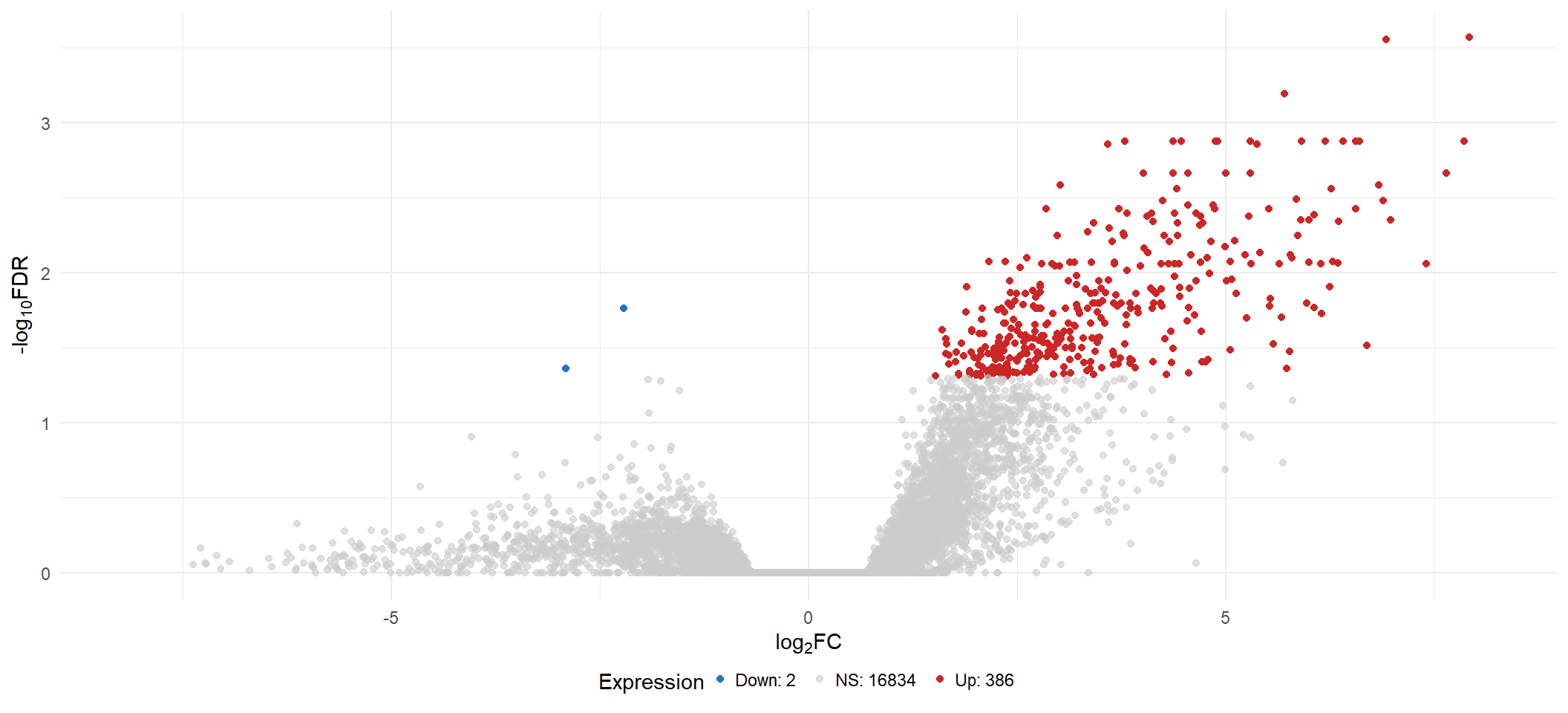

Version	Author	Date
b44640a	Ha Manh Tran	2023-01-23
d578f46	Ha Manh Tran	2023-01-21
159f352	tranmanhha135	2023-01-21
3119fad	tranmanhha135	2022-11-05

Top Upregulated

heat_up[[3]]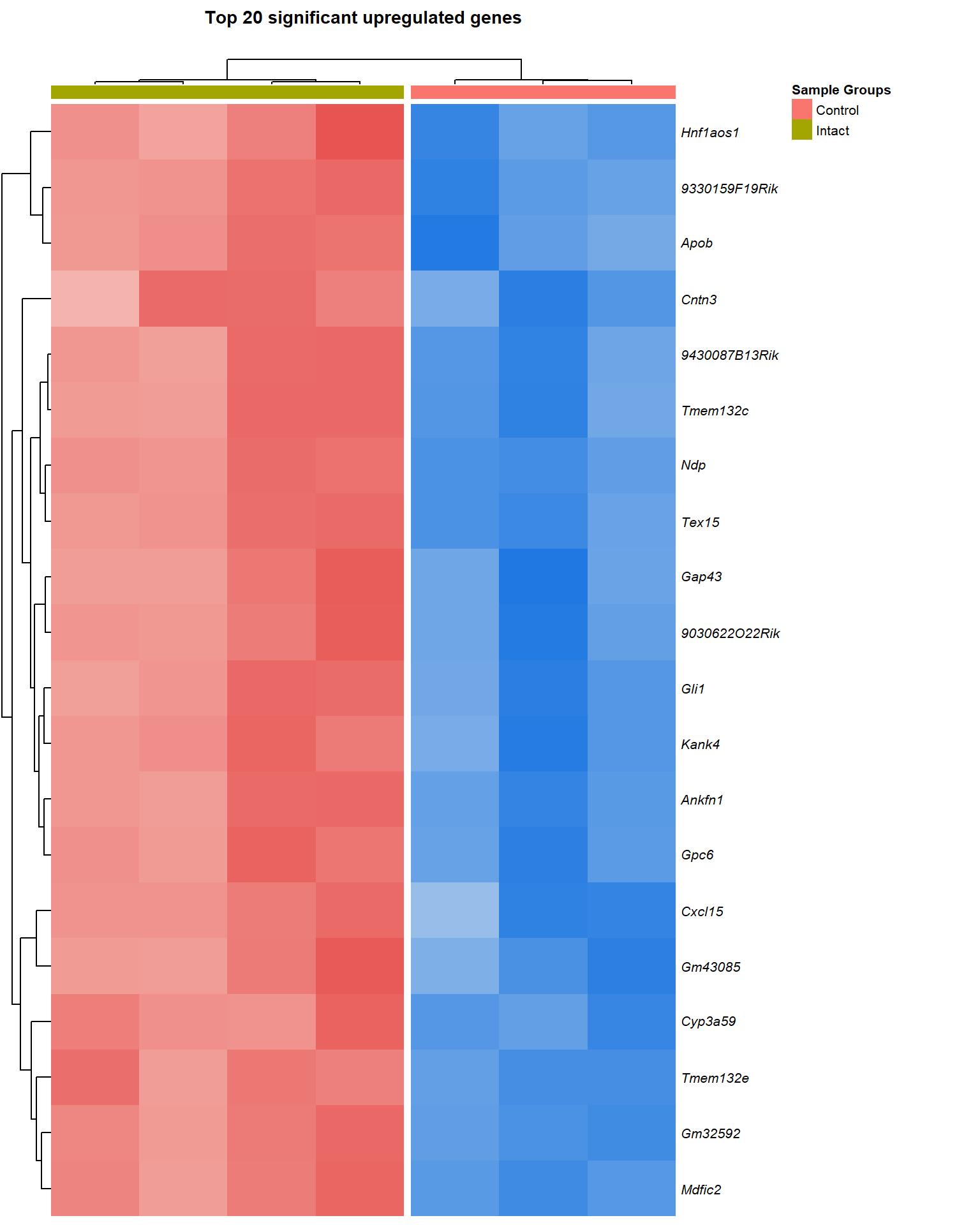

Version	Author	Date
d578f46	Ha Manh Tran	2023-01-21
159f352	tranmanhha135	2023-01-21
691cf34	Ha Manh Tran	2023-01-20
3119fad	tranmanhha135	2022-11-05

Top Downregulated

heat_down[[3]]

Version	Author	Date
d578f46	Ha Manh Tran	2023-01-21
159f352	tranmanhha135	2023-01-21
691cf34	Ha Manh Tran	2023-01-20
3119fad	tranmanhha135	2022-11-05

Export

# export toptable for Dexter rewrite

## First paper (suitable # of DE genes for INT vs CONT)
writexl::write_xlsx(x = lmTreat_fc1.5_voom2_fdr0.05, here::here("3_output/lmTreat_fc1.5_voom2_all_fdr.xlsx"))
## Second paper (suitable # of DE genes for INT vs SVS_VAS, SVX vs SVX_VAS, and VAS vs SVX_VAS)
# writexl::write_xlsx(x = lm_voom2_pval0.01, here::here("3_output/lm_voom2_all.xlsx"))

# export excel spreadsheet
writexl::write_xlsx(x = lmTreat_all, here::here("3_output/lmTreat_all.xlsx"))
writexl::write_xlsx(x = lmTreat_sig, here::here("3_output/lmTreat_sig.xlsx"))

# save RDS object for enrichment analysis
saveRDS(object = fc, file = here::here("0_data/RDS_objects/fc.rds"))
saveRDS(object = lfc, file = here::here("0_data/RDS_objects/lfc.rds"))
saveRDS(object = lmTreat, file = here::here("0_data/RDS_objects/lmTreat.rds"))
saveRDS(object = lmTreat_all, file = here::here("0_data/RDS_objects/lmTreat_all.rds"))
saveRDS(object = lmTreat_sig, file = here::here("0_data/RDS_objects/lmTreat_sig.rds"))

sessionInfo()

R version 4.3.1 (2023-06-16 ucrt)
Platform: x86_64-w64-mingw32/x64 (64-bit)
Running under: Windows 10 x64 (build 19045)

Matrix products: default


locale:
[1] LC_COLLATE=English_Australia.utf8  LC_CTYPE=English_Australia.utf8   
[3] LC_MONETARY=English_Australia.utf8 LC_NUMERIC=C                      
[5] LC_TIME=English_Australia.utf8    

time zone: Australia/Adelaide
tzcode source: internal

attached base packages:
[1] grid      stats     graphics  grDevices utils     datasets  methods  
[8] base     

other attached packages:
 [1] Glimma_2.10.0     edgeR_3.42.4      limma_3.56.2      viridis_0.6.4    
 [5] viridisLite_0.4.2 ggrepel_0.9.3     ggpubr_0.6.0      ggplotify_0.1.2  
 [9] DT_0.29           pheatmap_1.0.12   cowplot_1.1.1     pander_0.6.5     
[13] kableExtra_1.3.4  lubridate_1.9.2   forcats_1.0.0     stringr_1.5.0    
[17] purrr_1.0.1       tidyr_1.3.0       ggplot2_3.4.3     tidyverse_2.0.0  
[21] reshape2_1.4.4    tibble_3.2.1      readr_2.1.4       magrittr_2.0.3   
[25] dplyr_1.1.2      

loaded via a namespace (and not attached):
  [1] bitops_1.0-7                gridExtra_2.3              
  [3] writexl_1.4.2               rlang_1.1.1                
  [5] git2r_0.32.0                matrixStats_1.0.0          
  [7] compiler_4.3.1              systemfonts_1.0.4          
  [9] vctrs_0.6.3                 rvest_1.0.3                
 [11] crayon_1.5.2                pkgconfig_2.0.3            
 [13] fastmap_1.1.1               ellipsis_0.3.2             
 [15] XVector_0.40.0              backports_1.4.1            
 [17] labeling_0.4.3              utf8_1.2.3                 
 [19] promises_1.2.0.1            rmarkdown_2.24             
 [21] tzdb_0.4.0                  ragg_1.2.5                 
 [23] xfun_0.39                   zlibbioc_1.46.0            
 [25] cachem_1.0.8                GenomeInfoDb_1.36.3        
 [27] jsonlite_1.8.7              highr_0.10                 
 [29] later_1.3.1                 DelayedArray_0.26.7        
 [31] BiocParallel_1.34.2         broom_1.0.5                
 [33] parallel_4.3.1              R6_2.5.1                   
 [35] bslib_0.5.1                 stringi_1.7.12             
 [37] RColorBrewer_1.1-3          car_3.1-2                  
 [39] GenomicRanges_1.52.0        jquerylib_0.1.4            
 [41] SummarizedExperiment_1.30.2 Rcpp_1.0.11                
 [43] knitr_1.44                  IRanges_2.34.1             
 [45] Matrix_1.6-1                httpuv_1.6.11              
 [47] timechange_0.2.0            tidyselect_1.2.0           
 [49] rstudioapi_0.15.0           abind_1.4-5                
 [51] yaml_2.3.7                  codetools_0.2-19           
 [53] lattice_0.21-8              plyr_1.8.8                 
 [55] Biobase_2.60.0              withr_2.5.0                
 [57] evaluate_0.21               gridGraphics_0.5-1         
 [59] xml2_1.3.5                  pillar_1.9.0               
 [61] MatrixGenerics_1.12.3       carData_3.0-5              
 [63] whisker_0.4.1               stats4_4.3.1               
 [65] generics_0.1.3              rprojroot_2.0.3            
 [67] RCurl_1.98-1.12             hms_1.1.3                  
 [69] S4Vectors_0.38.1            munsell_0.5.0              
 [71] scales_1.2.1                glue_1.6.2                 
 [73] tools_4.3.1                 locfit_1.5-9.8             
 [75] webshot_0.5.5               ggsignif_0.6.4             
 [77] fs_1.6.3                    crosstalk_1.2.0            
 [79] colorspace_2.1-0            GenomeInfoDbData_1.2.10    
 [81] cli_3.6.1                   textshaping_0.3.6          
 [83] workflowr_1.7.1             fansi_1.0.4                
 [85] S4Arrays_1.0.6              svglite_2.1.1              
 [87] gtable_0.3.4                rstatix_0.7.2              
 [89] yulab.utils_0.0.9           DESeq2_1.40.2              
 [91] sass_0.4.7                  digest_0.6.33              
 [93] BiocGenerics_0.46.0         farver_2.1.1               
 [95] htmlwidgets_1.6.2           memoise_2.0.1              
 [97] htmltools_0.5.5             lifecycle_1.0.3            
 [99] here_1.0.1                  httr_1.4.7

DGE Analysis

Ha M. Tran

22/08/2021

Data Setup

Import DGElist Data

Initial Parameterisation

Design Matrix

Contrast Matrix

Limma-Voom

Apply voom transformation

Observational level weights

Observational & group level weights

Observational & sample level weights

Apply linear model

Without TREAT

TREAT FC=1.05

TREAT FC=1.1

TREAT FC=1.5

Differential Gene Expression analysis

TREAT FC= 1.05

P Value histogram

MA Plot

Volcano Plot

Top Upregulated

Top Downregulated

TREAT FC= 1.1

P Value histogram

MA Plot

Volcano Plot

Top Upregulated

Top Downregulated

TREAT FC= 1.5

P Value histogram

MA Plot

Volcano Plot

Top Upregulated

Top Downregulated

Export