GO Analysis

workflowr

• Summary
• Checks
• Past versions

Last updated: 2023-09-16

Checks: 7 0

Knit directory: Mouse_endometrial_transcriptome_2023/1_analysis/

This reproducible R Markdown analysis was created with workflowr (version 1.7.1). The Checks tab describes the reproducibility checks that were applied when the results were created. The Past versions tab lists the development history.

---

R Markdown file: up-to-date

Great! Since the R Markdown file has been committed to the Git repository, you know the exact version of the code that produced these results.

Environment: empty

Great job! The global environment was empty. Objects defined in the global environment can affect the analysis in your R Markdown file in unknown ways. For reproduciblity it’s best to always run the code in an empty environment.

Seed: set.seed(12345)

The command set.seed(12345) was run prior to running the code in the R Markdown file. Setting a seed ensures that any results that rely on randomness, e.g. subsampling or permutations, are reproducible.

Session information: recorded

Great job! Recording the operating system, R version, and package versions is critical for reproducibility.

Cache: none

Nice! There were no cached chunks for this analysis, so you can be confident that you successfully produced the results during this run.

File paths: relative

Great job! Using relative paths to the files within your workflowr project makes it easier to run your code on other machines.

Repository version: 18c6463

Great! You are using Git for version control. Tracking code development and connecting the code version to the results is critical for reproducibility.

The results in this page were generated with repository version 18c6463. See the Past versions tab to see a history of the changes made to the R Markdown and HTML files.

Note that you need to be careful to ensure that all relevant files for the analysis have been committed to Git prior to generating the results (you can use wflow_publish or wflow_git_commit). workflowr only checks the R Markdown file, but you know if there are other scripts or data files that it depends on. Below is the status of the Git repository when the results were generated:

Ignored files:
    Ignored:    .Rproj.user/

Untracked files:
    Untracked:  .gitignore
    Untracked:  0_data/RDS_objects/DT.rds

Unstaged changes:
    Modified:   0_data/RDS_objects/dge.rds
    Modified:   0_data/RDS_objects/enrichGO.rds
    Modified:   0_data/RDS_objects/enrichGO_sig.rds
    Modified:   0_data/RDS_objects/fc.rds
    Modified:   0_data/RDS_objects/lfc.rds
    Modified:   0_data/RDS_objects/lmTreat.rds
    Modified:   0_data/RDS_objects/lmTreat_all.rds
    Modified:   0_data/RDS_objects/lmTreat_sig.rds
    Modified:   0_data/RDS_objects/pub.rds
    Deleted:    1_analysis/mmu04060.pv.png
    Deleted:    1_analysis/mmu04151.pv.png
    Deleted:    1_analysis/mmu04270.pv.png
    Deleted:    1_analysis/mmu04510.pv.png
    Deleted:    1_analysis/mmu04640.pv.png
    Deleted:    1_analysis/mmu04670.pv.png
    Modified:   2_plots/de/pval_1.05.svg
    Modified:   2_plots/de/pval_1.1.svg
    Modified:   2_plots/de/pval_1.5.svg
    Modified:   2_plots/go/bp_dot_1.05.svg
    Modified:   2_plots/go/bp_dot_1.5.svg
    Modified:   2_plots/go/cc_dot_1.05.svg
    Modified:   2_plots/go/cc_dot_1.5.svg
    Modified:   2_plots/go/mf_dot_1.5.svg
    Modified:   2_plots/go/upset_1.05.svg
    Modified:   2_plots/go/upset_1.1.svg
    Modified:   2_plots/go/upset_1.5.svg
    Modified:   2_plots/ipa/Cell-To-Cell Signaling.svg
    Modified:   2_plots/ipa/diseaseAndFunction.svg
    Modified:   2_plots/ipa/pathways.svg
    Modified:   2_plots/kegg/kegg_dot_1.05.svg
    Modified:   2_plots/kegg/kegg_dot_1.1.svg
    Modified:   2_plots/kegg/kegg_dot_1.5.svg
    Modified:   2_plots/kegg/upset_kegg_1.05.svg
    Modified:   2_plots/kegg/upset_kegg_1.1.svg
    Modified:   2_plots/kegg/upset_kegg_1.5.svg
    Modified:   2_plots/qc/PCA_IntvsCont.svg
    Modified:   2_plots/qc/counts_after_filtering_3_3.svg
    Modified:   2_plots/qc/counts_before_after_filtering_3_3.svg
    Modified:   2_plots/qc/counts_before_filtering.svg
    Modified:   2_plots/qc/library_size.svg
    Modified:   2_plots/reactome/react_dot_1.05.svg
    Modified:   2_plots/reactome/react_dot_1.1.svg
    Modified:   2_plots/reactome/react_dot_1.5.svg
    Modified:   2_plots/reactome/upset_react_1.05.svg
    Modified:   2_plots/reactome/upset_react_1.1.svg
    Modified:   2_plots/reactome/upset_react_1.5.svg
    Modified:   3_output/enrichGO_sig.xlsx
    Modified:   3_output/enrichKEGG_all.xlsx
    Modified:   3_output/enrichKEGG_sig.xlsx
    Modified:   3_output/lmTreat_all.xlsx
    Modified:   3_output/lmTreat_fc1.5_voom2_all_fdr.xlsx
    Modified:   3_output/lmTreat_sig.xlsx
    Modified:   3_output/reactome_all.xlsx
    Modified:   3_output/reactome_sig.xlsx

Note that any generated files, e.g. HTML, png, CSS, etc., are not included in this status report because it is ok for generated content to have uncommitted changes.

---

These are the previous versions of the repository in which changes were made to the R Markdown (1_analysis/go.Rmd) and HTML (docs/go.html) files. If you’ve configured a remote Git repository (see ?wflow_git_remote), click on the hyperlinks in the table below to view the files as they were in that past version.

File	Version	Author	Date	Message
Rmd	18c6463	Ha Manh Tran	2023-09-16	Added KEGG copyright permission and changed kable
html	b44640a	Ha Manh Tran	2023-01-23	Build site.
Rmd	eb10bef	Ha Manh Tran	2023-01-22	workflowr::wflow_publish(here::here("1_analysis/*.Rmd"))
html	8c9178d	tranmanhha135	2023-01-21	added png
html	d578f46	Ha Manh Tran	2023-01-21	Build site.
html	159f352	tranmanhha135	2023-01-21	adding for pathview
Rmd	4d51a4e	tranmanhha135	2023-01-20	test png
html	4d51a4e	tranmanhha135	2023-01-20	test png
html	691cf34	Ha Manh Tran	2023-01-20	Build site.
Rmd	7f6bab2	Ha Manh Tran	2023-01-20	workflowr::wflow_publish(here::here("1_analysis/*.Rmd"))
Rmd	b6cf190	tranmanhha135	2023-01-19	quick commit
Rmd	3119fad	tranmanhha135	2022-11-05	build website
html	3119fad	tranmanhha135	2022-11-05	build website

---

Data Setup

# working with data
library(dplyr)
library(magrittr)
library(readr)
library(tibble)
library(reshape2)
library(tidyverse)

# Visualisation:
library(kableExtra)
library(ggplot2)
library(grid)
library(DT)

# Custom ggplot
library(gridExtra)
library(ggbiplot)
library(ggrepel)


# Bioconductor packages:
library(edgeR)
library(limma)
library(Glimma)
library(clusterProfiler)
library(org.Mm.eg.db)
library(enrichplot)

theme_set(theme_minimal())
pub <- readRDS(here::here("0_data/RDS_objects/pub.rds"))
DT <- readRDS(here::here("0_data/RDS_objects/DT.rds"))

Import DGElist Data

DGElist object containing the raw feature count, sample metadata, and gene metadata, created in the Set Up stage.

# load DGElist previously created in the set up
dge <- readRDS(here::here("0_data/RDS_objects/dge.rds"))
fc <- readRDS(here::here("0_data/RDS_objects/fc.rds"))
lfc <- readRDS(here::here("0_data/RDS_objects/lfc.rds"))
lmTreat <- readRDS(here::here("0_data/RDS_objects/lmTreat.rds"))
lmTreat_sig <- readRDS(here::here("0_data/RDS_objects/lmTreat_sig.rds"))

GO Analysis

goSummaries is a package created by Dr Stephen Pederson for filtering GO terms based on ontology level.

# circumvent rerunning of lengthy analysis.
enrichGO <- readRDS(here::here("0_data/RDS_objects/enrichGO.rds"))
enrichGO_sig <- readRDS(here::here("0_data/RDS_objects/enrichGO_sig.rds"))

# download go summaries and set the minimum ontology level
goSummaries <- url("https://uofabioinformaticshub.github.io/summaries2GO/data/goSummaries.RDS") %>%
  readRDS()
minPath <- 3

enrichGO=list()
enrichGO_sig <- list()
for (i in 1:length(fc)) {
  x <- fc[i] %>% as.character()
  # find enriched GO terms
  enrichGO[[x]] <- clusterProfiler::enrichGO(
    gene = lmTreat_sig[[x]]$entrezid,
    OrgDb = org.Mm.eg.db,
    keyType = "ENTREZID",
    ont = "ALL",
    pAdjustMethod = "fdr",
    pvalueCutoff = 0.05
  )

  # bind to goSummaries to elminate go terms with ontology levels 1 and 2.
  enrichGO_sig[[x]] <- enrichGO[[x]] %>% 
    clusterProfiler::setReadable(OrgDb = org.Mm.eg.db, keyType = "auto")

  enrichGO_sig[[x]] <- enrichGO_sig[[x]] %>%
    as.data.frame() %>%
    rownames_to_column("id") %>%
    left_join(goSummaries) %>%
    dplyr::filter(shortest_path >= minPath) %>%
    column_to_rownames("id")

  # adjust go results, separate compound column, add FDR column, adjust the GeneRatio column
  enrichGO_sig[[x]] <- enrichGO_sig[[x]] %>%
    separate(col = BgRatio, sep = "/", into = c("Total", "Universe")) %>%
    dplyr::mutate(
      logFDR = -log(p.adjust, 10),
      GeneRatio = Count / as.numeric(Total)) %>% 
    dplyr::select(c("Description", "ontology", "GeneRatio", "pvalue", "p.adjust", "logFDR", "qvalue", "geneID", "Count"))
  
  # at the beginnning of a word (after 35 characters), add a newline. shorten the y axis for dot plot 
  # enrichGO_sig[[x]]$Description <- sub(pattern = "(.{1,35})(?:$| )", 
  #                                      replacement = "\\1\n", 
  #                                      x = enrichGO_sig[[x]]$Description)
  
  # # remove the additional newline at the end of the string
  # enrichGO_sig[[x]]$Description <- sub(pattern = "\n$", 
  #                                      replacement = "", 
  #                                      x = enrichGO_sig[[x]]$Description)
}

FC=1.05

# display the top 30 most sig
enrichGO_sig[[1]] %>% 
  dplyr::mutate_if(is.numeric, funs(as.character(signif(.,3)))) %>% 
  DT(., caption = "Significantly enriched GO terms")

  # kable(caption = "Significantly enriched GO terms") %>%
  # kable_styling(bootstrap_options = c("striped", "hover")) %>%
  # scroll_box(height = "600px")

Visualisation

bp_dot=list()
mf_dot=list()
cc_dot=list()
upset=list()
for (i in 1:length(fc)) {
  x <- fc[i] %>% as.character()
  
  # extract the enriched GO terms from each ontology
  bp <- enrichGO_sig[[x]] %>% dplyr::filter(ontology == "BP") 
  mf <- enrichGO_sig[[x]] %>% dplyr::filter(ontology == "MF")
  cc <- enrichGO_sig[[x]] %>% dplyr::filter(ontology == "CC")

  # bp dot plot, save
  bp_dot[[x]] <- ggplot(bp[1:15, ]) +
    geom_point(aes(x = GeneRatio, y = reorder(Description, GeneRatio), colour = logFDR, size = Count)) +
    scale_color_gradient(low = "dodgerblue3", high = "firebrick3", limits = c(0, NA)) +
    scale_size(range = c(.5,3)) +
    ggtitle("Biological Process") +
    ylab(label = "") +
    xlab(label = "Gene Ratio") +
    labs(color = expression("-log"[10] * "FDR"), size = "Gene Counts")
  ggsave(filename = paste0("bp_dot_", fc[i], ".svg"), plot = bp_dot[[x]] + pub, path = here::here("2_plots/go/"), 
         width = 200, height = 120, units = "mm")

  # mf dot plot, save
  mf_dot[[x]] <- ggplot(mf[1:15, ]) +
    geom_point(aes(x = GeneRatio, y = reorder(Description, GeneRatio), colour = logFDR, size = Count)) +
    scale_color_gradient(low = "dodgerblue3", high = "firebrick3", limits = c(0, NA)) +
    scale_size(range = c(.5,3)) +
    ggtitle("Molecular Function") +
    ylab(label = "") +
    xlab(label = "Gene Ratio") +
    labs(color = expression("-log"[10] * "FDR"), size = "Gene Counts")
  ggsave(filename = paste0("mf_dot_", fc[i], ".svg"), plot = mf_dot[[x]] + pub, path = here::here("2_plots/go/"), 
         width = 200, height = 120, units = "mm")

  # cc dot plot, save
  cc_dot[[x]] <- ggplot(cc[1:15, ]) +
    geom_point(aes(x = GeneRatio, y = reorder(Description, GeneRatio), colour = logFDR, size = Count)) +
    scale_color_gradient(low = "dodgerblue3", high = "firebrick3", limits = c(0, NA)) +
    scale_size(range = c(.5,3)) +
    ggtitle("Cellular Components") +
    ylab(label = "") +
    xlab(label = "Gene Ratio") +
    labs(color = expression("-log"[10] * "FDR"), size = "Gene Counts")
  ggsave(filename = paste0("cc_dot_", fc[i], ".svg"), plot = cc_dot[[x]] + pub, path = here::here("2_plots/go/"), 
         width = 200, height = 120, units = "mm")
  
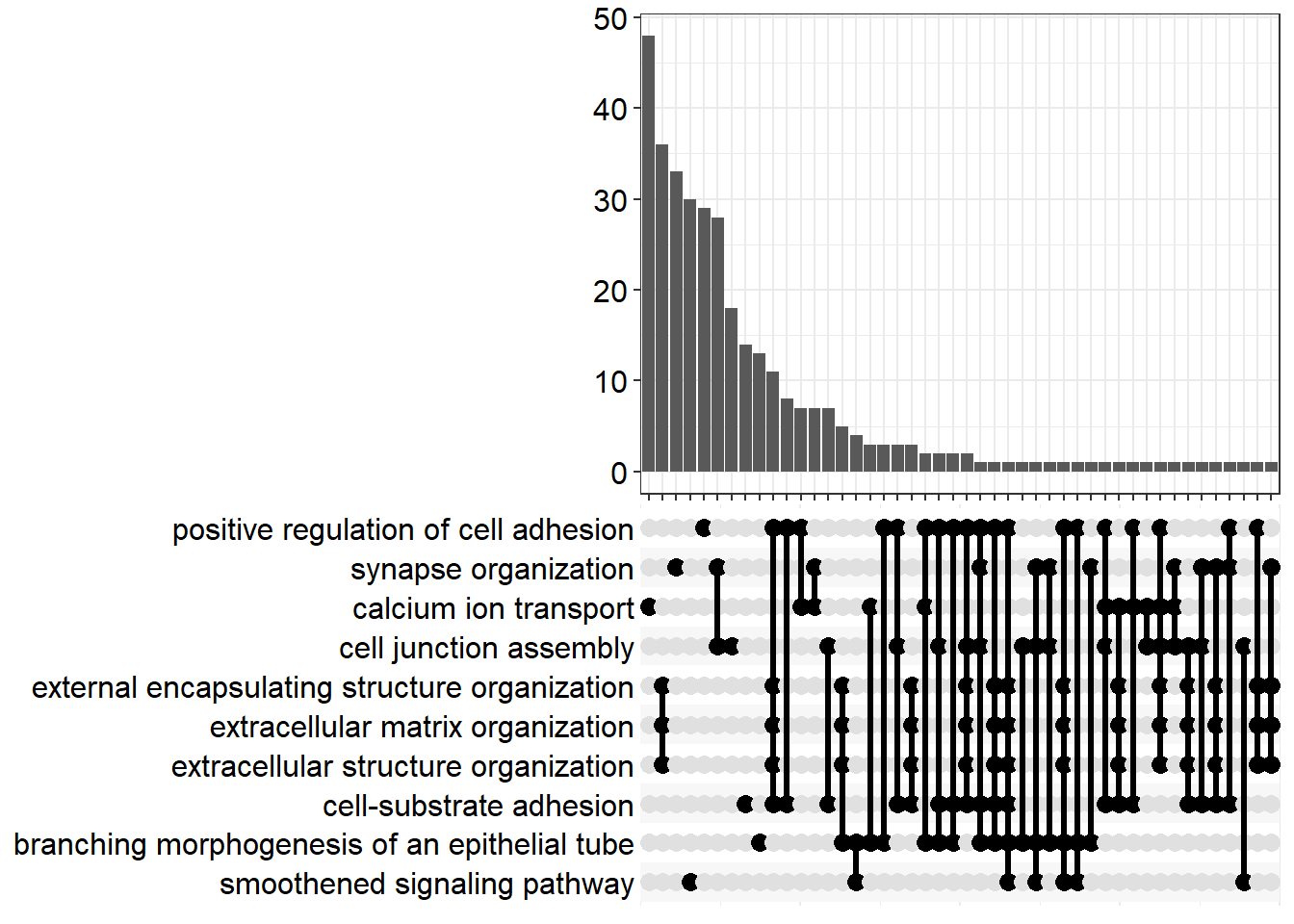
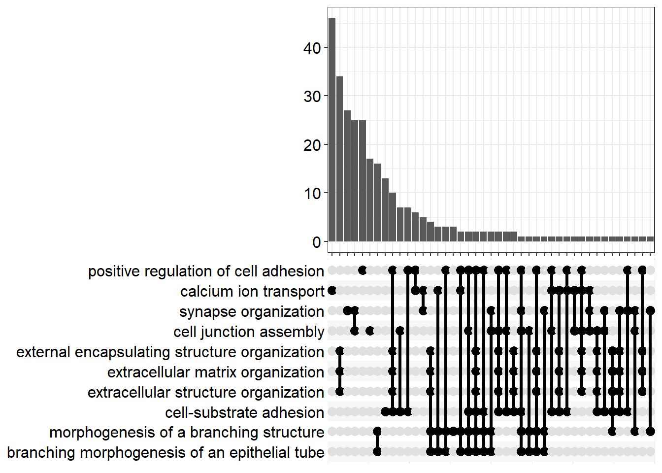
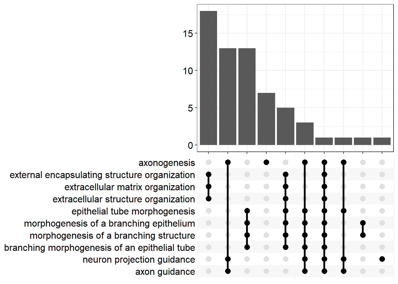
  upset[[x]] <- upsetplot(x = enrichGO[[x]], 10)
  ggsave(filename = paste0("upset_", fc[i], ".svg"), plot = upset[[x]], path = here::here("2_plots/go/"), width = 250, height = 166, units = "mm")
}

Biological Process

bp_dot[[1]]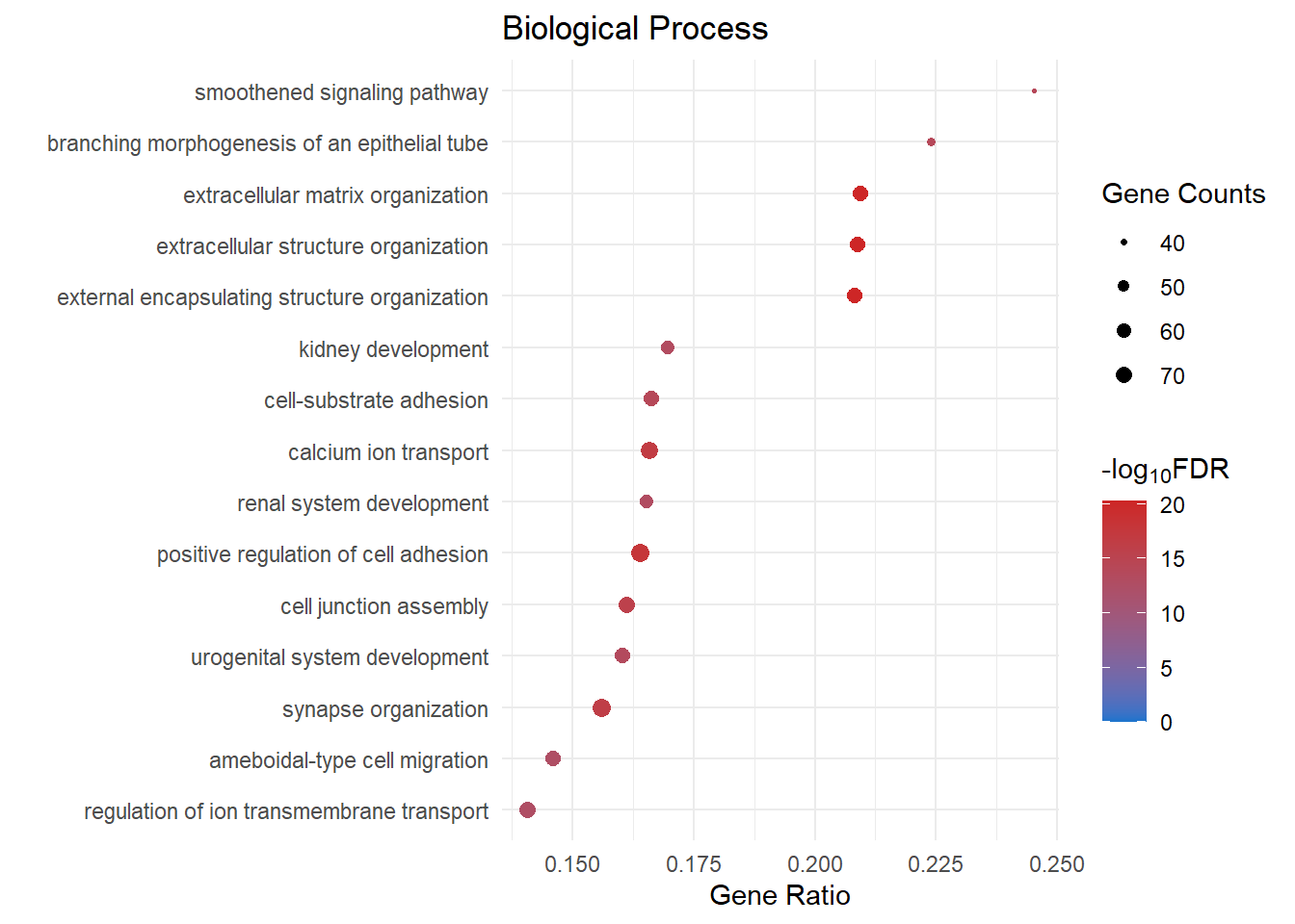 

Past versions of unnamed-chunk-3-1.png

Version	Author	Date
d578f46	Ha Manh Tran	2023-01-21
159f352	tranmanhha135	2023-01-21
4d51a4e	tranmanhha135	2023-01-20
691cf34	Ha Manh Tran	2023-01-20
3119fad	tranmanhha135	2022-11-05

Molecular Function

mf_dot[[1]]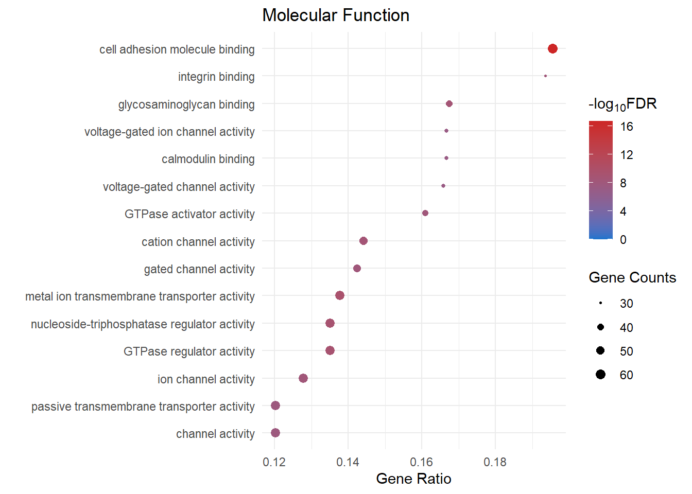

Past versions of unnamed-chunk-4-1.png

Version	Author	Date
d578f46	Ha Manh Tran	2023-01-21
159f352	tranmanhha135	2023-01-21
4d51a4e	tranmanhha135	2023-01-20
691cf34	Ha Manh Tran	2023-01-20
3119fad	tranmanhha135	2022-11-05

Cellular Components

cc_dot[[1]]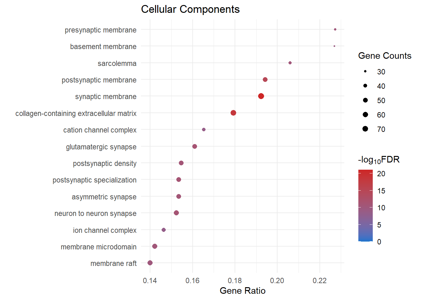

Past versions of unnamed-chunk-5-1.png

Version	Author	Date
d578f46	Ha Manh Tran	2023-01-21
159f352	tranmanhha135	2023-01-21
4d51a4e	tranmanhha135	2023-01-20
691cf34	Ha Manh Tran	2023-01-20
3119fad	tranmanhha135	2022-11-05

Upset

upset[[1]]

Past versions of unnamed-chunk-6-1.png

Version	Author	Date
d578f46	Ha Manh Tran	2023-01-21
159f352	tranmanhha135	2023-01-21
691cf34	Ha Manh Tran	2023-01-20
3119fad	tranmanhha135	2022-11-05

FC=1.1

# display the top 30 most sig
enrichGO_sig[[2]] %>% 
  dplyr::mutate_if(is.numeric, funs(as.character(signif(.,3)))) %>%
  DT(.,caption = "Significantly enriched GO terms")

  # kable(caption = "Significantly enriched GO terms") %>%
  # kable_styling(bootstrap_options = c("striped", "hover")) %>%
  # scroll_box(height = "600px")

Visualisation

Biological Process

bp_dot[[2]]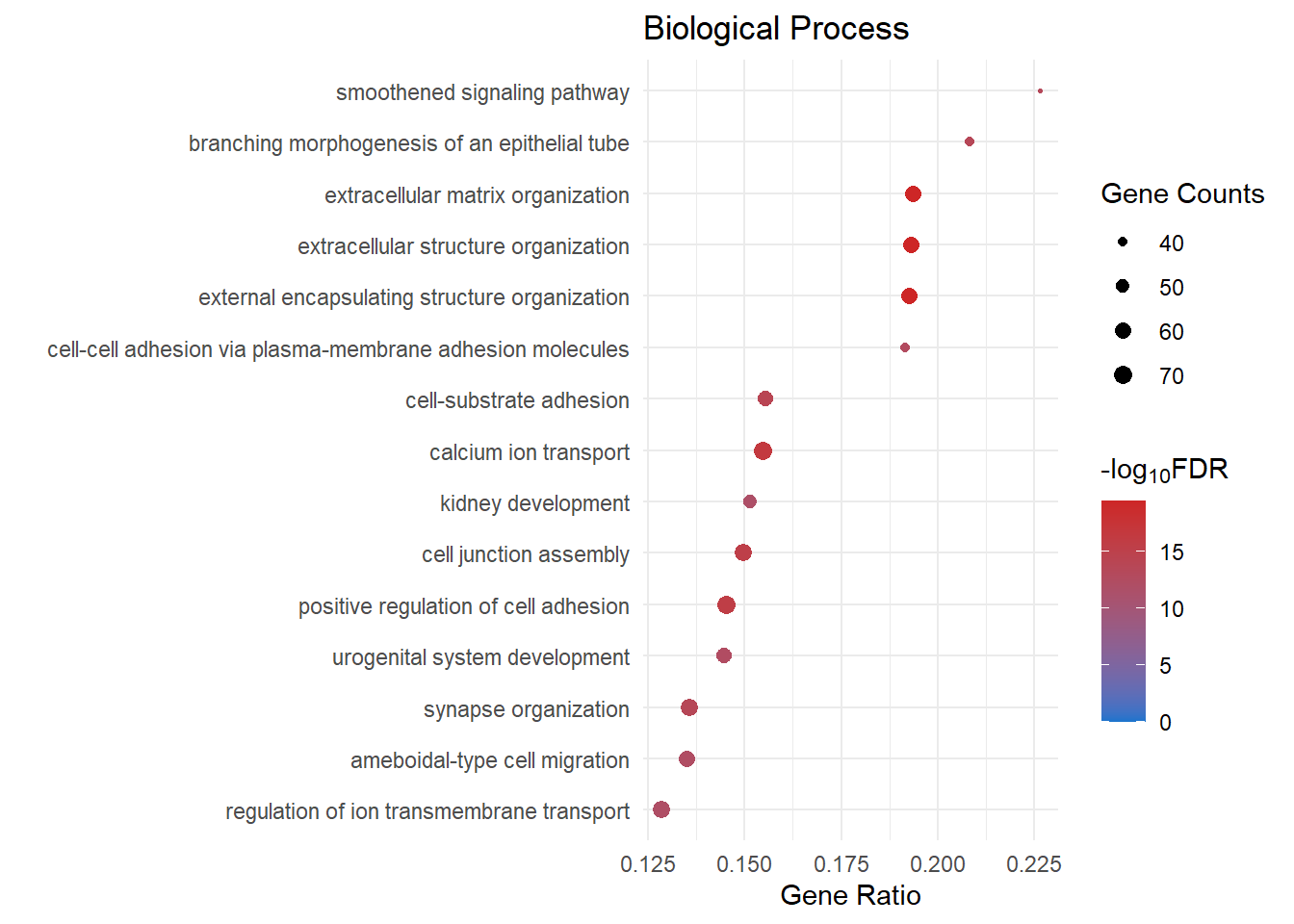

Past versions of unnamed-chunk-8-1.png

Version	Author	Date
d578f46	Ha Manh Tran	2023-01-21
159f352	tranmanhha135	2023-01-21
4d51a4e	tranmanhha135	2023-01-20
691cf34	Ha Manh Tran	2023-01-20
3119fad	tranmanhha135	2022-11-05

Molecular Function

mf_dot[[2]]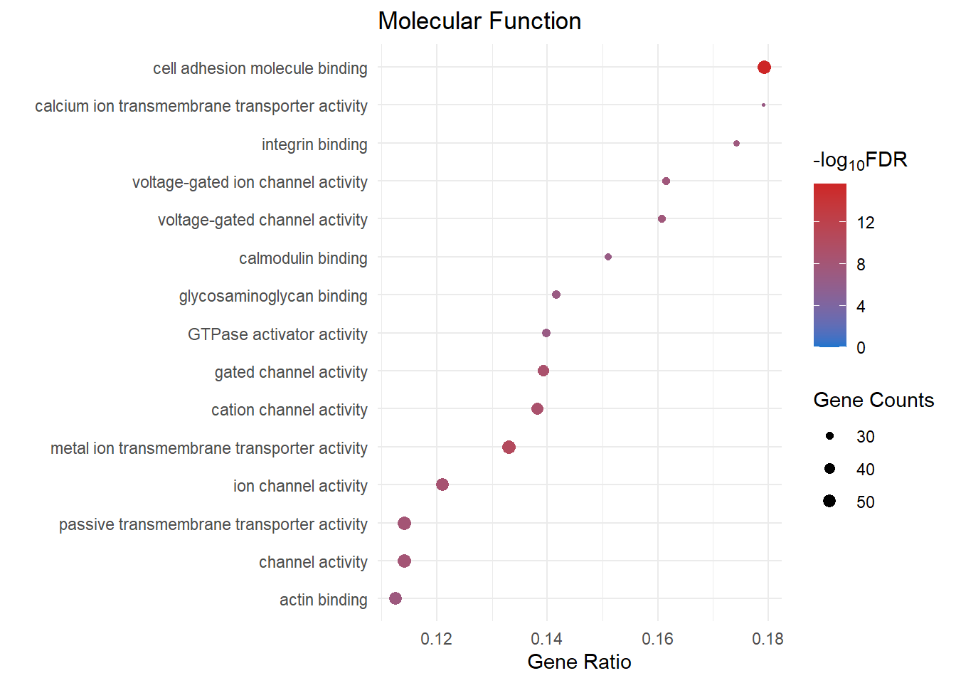

Past versions of unnamed-chunk-9-1.png

Version	Author	Date
d578f46	Ha Manh Tran	2023-01-21
159f352	tranmanhha135	2023-01-21
4d51a4e	tranmanhha135	2023-01-20
691cf34	Ha Manh Tran	2023-01-20
3119fad	tranmanhha135	2022-11-05

Cellular Components

cc_dot[[2]]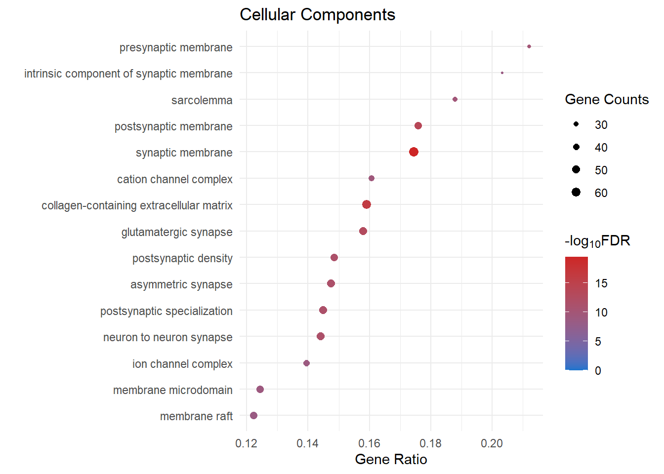

Past versions of unnamed-chunk-10-1.png

Version	Author	Date
d578f46	Ha Manh Tran	2023-01-21
159f352	tranmanhha135	2023-01-21
4d51a4e	tranmanhha135	2023-01-20
691cf34	Ha Manh Tran	2023-01-20
3119fad	tranmanhha135	2022-11-05

Upset

upset[[2]]

Past versions of unnamed-chunk-11-1.png

Version	Author	Date
d578f46	Ha Manh Tran	2023-01-21
159f352	tranmanhha135	2023-01-21
691cf34	Ha Manh Tran	2023-01-20
3119fad	tranmanhha135	2022-11-05

FC=1.5

# display the top 30 most sig
enrichGO_sig[[3]] %>% 
  dplyr::mutate_if(is.numeric, funs(as.character(signif(.,3)))) %>%
  DT(.,caption = "Significantly enriched GO terms") 

  # kable(caption = "Significantly enriched GO terms") %>%
  # kable_styling(bootstrap_options = c("striped", "hover")) %>%
  # scroll_box(height = "600px")

Visualisation

Biological Process

bp_dot[[3]]

Past versions of unnamed-chunk-13-1.png

Version	Author	Date
d578f46	Ha Manh Tran	2023-01-21
159f352	tranmanhha135	2023-01-21
4d51a4e	tranmanhha135	2023-01-20
691cf34	Ha Manh Tran	2023-01-20
3119fad	tranmanhha135	2022-11-05

Molecular Function

mf_dot[[3]]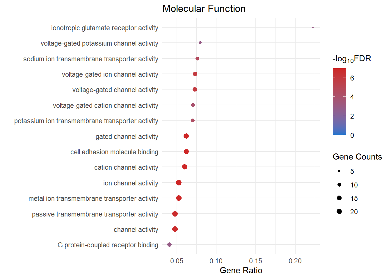

Past versions of unnamed-chunk-14-1.png

Version	Author	Date
d578f46	Ha Manh Tran	2023-01-21
159f352	tranmanhha135	2023-01-21
4d51a4e	tranmanhha135	2023-01-20
691cf34	Ha Manh Tran	2023-01-20
3119fad	tranmanhha135	2022-11-05

Cellular Components

cc_dot[[3]]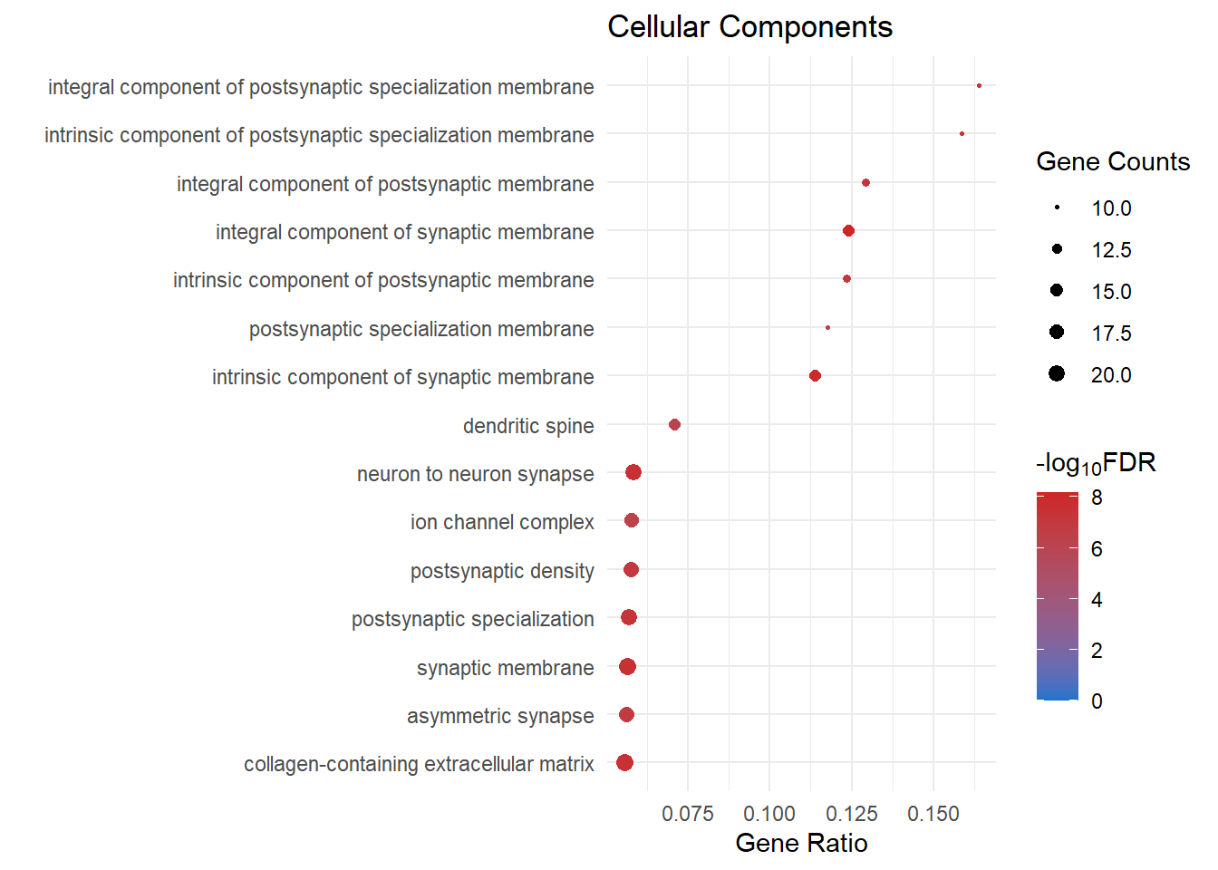

Past versions of unnamed-chunk-15-1.png

Version	Author	Date
d578f46	Ha Manh Tran	2023-01-21
159f352	tranmanhha135	2023-01-21
4d51a4e	tranmanhha135	2023-01-20
691cf34	Ha Manh Tran	2023-01-20
3119fad	tranmanhha135	2022-11-05

Upset

upset[[3]]

Past versions of unnamed-chunk-16-1.png

Version	Author	Date
d578f46	Ha Manh Tran	2023-01-21
159f352	tranmanhha135	2023-01-21
691cf34	Ha Manh Tran	2023-01-20
3119fad	tranmanhha135	2022-11-05

Export Data

# save to excel
writexl::write_xlsx(x = enrichGO_sig, here::here("3_output/enrichGO_sig.xlsx"))
saveRDS(object = enrichGO_sig,file = here::here("0_data/RDS_objects/enrichGO_sig.rds"))
saveRDS(object = enrichGO,file = here::here("0_data/RDS_objects/enrichGO.rds"))

Session information

sessionInfo()

R version 4.3.1 (2023-06-16 ucrt)
Platform: x86_64-w64-mingw32/x64 (64-bit)
Running under: Windows 10 x64 (build 19045)

Matrix products: default


locale:
[1] LC_COLLATE=English_Australia.utf8  LC_CTYPE=English_Australia.utf8   
[3] LC_MONETARY=English_Australia.utf8 LC_NUMERIC=C                      
[5] LC_TIME=English_Australia.utf8    

time zone: Australia/Adelaide
tzcode source: internal

attached base packages:
[1] stats4    grid      stats     graphics  grDevices utils     datasets 
[8] methods   base     

other attached packages:
 [1] enrichplot_1.20.1     org.Mm.eg.db_3.17.0   AnnotationDbi_1.62.2 
 [4] IRanges_2.34.1        S4Vectors_0.38.1      Biobase_2.60.0       
 [7] BiocGenerics_0.46.0   clusterProfiler_4.8.3 Glimma_2.10.0        
[10] edgeR_3.42.4          limma_3.56.2          ggrepel_0.9.3        
[13] ggbiplot_0.55         scales_1.2.1          plyr_1.8.8           
[16] gridExtra_2.3         DT_0.29               kableExtra_1.3.4     
[19] lubridate_1.9.2       forcats_1.0.0         stringr_1.5.0        
[22] purrr_1.0.1           tidyr_1.3.0           ggplot2_3.4.3        
[25] tidyverse_2.0.0       reshape2_1.4.4        tibble_3.2.1         
[28] readr_2.1.4           magrittr_2.0.3        dplyr_1.1.2          

loaded via a namespace (and not attached):
  [1] splines_4.3.1               later_1.3.1                
  [3] bitops_1.0-7                ggplotify_0.1.2            
  [5] polyclip_1.10-4             lifecycle_1.0.3            
  [7] rprojroot_2.0.3             lattice_0.21-8             
  [9] MASS_7.3-60                 crosstalk_1.2.0            
 [11] sass_0.4.7                  rmarkdown_2.24             
 [13] jquerylib_0.1.4             yaml_2.3.7                 
 [15] httpuv_1.6.11               cowplot_1.1.1              
 [17] DBI_1.1.3                   RColorBrewer_1.1-3         
 [19] abind_1.4-5                 zlibbioc_1.46.0            
 [21] rvest_1.0.3                 GenomicRanges_1.52.0       
 [23] ggraph_2.1.0                RCurl_1.98-1.12            
 [25] yulab.utils_0.0.9           tweenr_2.0.2               
 [27] git2r_0.32.0                GenomeInfoDbData_1.2.10    
 [29] tidytree_0.4.5              svglite_2.1.1              
 [31] codetools_0.2-19            DelayedArray_0.26.7        
 [33] DOSE_3.26.1                 xml2_1.3.5                 
 [35] ggforce_0.4.1               tidyselect_1.2.0           
 [37] aplot_0.2.1                 farver_2.1.1               
 [39] viridis_0.6.4               matrixStats_1.0.0          
 [41] webshot_0.5.5               jsonlite_1.8.7             
 [43] ellipsis_0.3.2              tidygraph_1.2.3            
 [45] systemfonts_1.0.4           tools_4.3.1                
 [47] treeio_1.24.3               ragg_1.2.5                 
 [49] Rcpp_1.0.11                 glue_1.6.2                 
 [51] xfun_0.39                   here_1.0.1                 
 [53] DESeq2_1.40.2               qvalue_2.32.0              
 [55] MatrixGenerics_1.12.3       GenomeInfoDb_1.36.3        
 [57] withr_2.5.0                 fastmap_1.1.1              
 [59] fansi_1.0.4                 digest_0.6.33              
 [61] timechange_0.2.0            R6_2.5.1                   
 [63] gridGraphics_0.5-1          textshaping_0.3.6          
 [65] colorspace_2.1-0            GO.db_3.17.0               
 [67] RSQLite_2.3.1               utf8_1.2.3                 
 [69] generics_0.1.3              data.table_1.14.8          
 [71] graphlayouts_1.0.0          httr_1.4.7                 
 [73] htmlwidgets_1.6.2           S4Arrays_1.0.6             
 [75] scatterpie_0.2.1            whisker_0.4.1              
 [77] pkgconfig_2.0.3             gtable_0.3.4               
 [79] blob_1.2.4                  workflowr_1.7.1            
 [81] XVector_0.40.0              shadowtext_0.1.2           
 [83] htmltools_0.5.5             fgsea_1.26.0               
 [85] ggupset_0.3.0               png_0.1-8                  
 [87] ggfun_0.1.3                 knitr_1.44                 
 [89] rstudioapi_0.15.0           tzdb_0.4.0                 
 [91] nlme_3.1-163                cachem_1.0.8               
 [93] parallel_4.3.1              HDO.db_0.99.1              
 [95] pillar_1.9.0                vctrs_0.6.3                
 [97] promises_1.2.0.1            evaluate_0.21              
 [99] cli_3.6.1                   locfit_1.5-9.8             
[101] compiler_4.3.1              rlang_1.1.1                
[103] crayon_1.5.2                labeling_0.4.3             
[105] fs_1.6.3                    writexl_1.4.2              
[107] stringi_1.7.12              viridisLite_0.4.2          
[109] BiocParallel_1.34.2         munsell_0.5.0              
[111] Biostrings_2.68.1           lazyeval_0.2.2             
[113] GOSemSim_2.26.1             Matrix_1.6-1               
[115] hms_1.1.3                   patchwork_1.1.3            
[117] bit64_4.0.5                 KEGGREST_1.40.0            
[119] SummarizedExperiment_1.30.2 igraph_1.5.1               
[121] memoise_2.0.1               bslib_0.5.1                
[123] ggtree_3.8.2                fastmatch_1.1-4            
[125] bit_4.0.5                   downloader_0.4             
[127] ape_5.7-1                   gson_0.1.0